This document is a quick introduction to MATLAB for image processing and analysis. It is more or less equal to the original tutorial, which can be found on a INF4300 resource site.

At the university, if you are on a Red Hat machine, MATLAB can be launched by the command matlab at the command prompt. In Windows there should be a MATLAB icon in the start-menu or on the desktop. For users without a matlab license and with no intention to getting one, there is an open-source alternative called Octave. Although they aim to be similar, there are situations where the two languages are not identical, and whenever matlab is referred here, it is the original matlab from MathWorks (unless otherwise stated).

Table of contents:

• Introduction to matlab
  • Set up
  • Matrices
  • Matrix operations
  • Control structures
  • The FIND function
  • Images
  • Image filtering

Set up

Make a folder named ‘INF2310’ and set this as the ‘current directory’ using the UI or using the MATLAB-function ‘cd’. When using the CD function and to use MATLAB more efficiently, the autocompletion is often handy. Activate it by hitting ‘Tab’. Save a copy of this file in that folder, and open it in MATLAB. To run a part of the code, select the code and hit F9. To run the selected block (the block with the caret), hit ‘Ctrl+Enter’. To run an entire file, you can:

• type the name of the file, e.g. ‘intro’, at the command prompt, or
• select the file and hit F9, or
• open the file and hit F5.

Matrices

The matrix $\begin{bmatrix} 1 & 0 & 0 \\ 0 & 1 & 0 \\ 0 & 0 & 1 \end{bmatrix}$ may be created like this:

someMatrix = [1 0 0 ; 0 1 0 ; 0 0 1]

e.g. [row1 ; row2 ; ... ; rowM], where a row can be defined as [number1 number2 ... numberN] or [number1, number2, ..., numberN].

MATLAB comes built-in with function for many common operations, for the case above we could have typed:

someMatrix = diag([1 1 1])

If you wonder how a function/operator works, type help <function name> or for (a sometimes more thorough) description in a separate window, type doc <function name>.

It is also possible to simply press F1 while the cursor is at a certain function to access MATLAB’s help for that particular funtion.

MATLAB matrices are dynamic objects, meaning one need not know the exact size of a matrix in advance. Initially a simple matrix can be made, and and later rows or colums may be added or removed. If, however, the size is known in advance and the matrix is large, it is wise to preallocate memory for the matrix before you start using it. This may greatly improve performance.

% Allocate memory for 100*100 matrix and fill it with 1's:
big_1 = ones(100); %<-- Terminating a line with ';' will suppress output.

% Or, allocate a 50*40*3 matrix and fill it with 0's:
big_0 = zeros([50 40 3]);

% A vector can be created using the '<from>:<step>:<to>' syntax:
steg1 = 1:2:50;

% The <step> is optional. If omitted the step defaults to 1:
steg2 = 1:50;

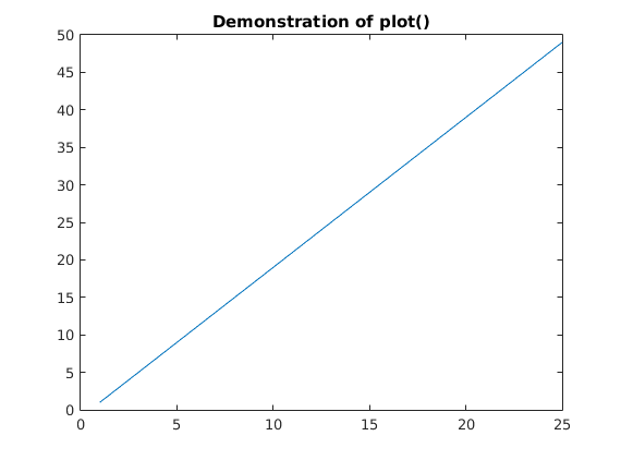
The standard plotting function is PLOT, e.g.:

plot(steg1);

An alternative is STEM. Look up how it works using ‘help stem’. You can add a title to the plot by using the title() function:

title('Demonstration of plot()');

Figure 1: Plot demonstration.

Extracting a value, or a series of values, from a matrix is easily achieved like this:

mat = [1 7 4 ; 3 4 5]
mat(2,1) % retrives the '3'

Note that matlab is an one-indexed language (like fortran), unlike languages like python and C/C++ which are zero-indexed

MATLAB lays out a column at a time in memory, hence the value 7 can either be retrieved using linear index:

mat(3)

or using (row,column)-index:

mat(1,2)

This is called column-major order, and it shares this way of putting values in memory with e.g. fortran and julia. Row-major order is the dual, and is used by e.g. C/C++ and numpy (python).

A range of elements may retrieved using the <from>:<to> syntax:

mat(1:2,1)     % First column
mat(1:end,1)   % The same, since n = 2
mat(:,1)       % The same, : is here 'all rows'

We can use the same syntax to set a range of elements:

mat(1:2,1:2) = 0

Note that a matrix can be stored in various formats, e.g. UINT8, INT8 or DOUBLE. They all have their conversion functions, see e.g. help uint8. If your result looks fishy, and you have a hard time figuring out why, a type conversion (of lack of one) may be the reason!

Matrix operations

Here we’ll demonstrate how some simple matrix operations is done in MATLAB

mat1 = [2 3; 5 7];
mat2 = [4 5; 1 9];

% Elementwise addition and subtraction.
mat1 + mat2
mat1 - mat2

% Transpose.
mat1.'
% Complex conjugate transpose (same as transpose when the matrix is real).
mat1'

% But notice the difference for a complex matrix
complexMatrix = [0 1i-2; 1i+2 0]

% Transpose for complex, see the function transpose
complexMatrix.'

% Complex conjugate transpose, see the function ctranspose
complexMatrix'

% Multiplication, division and power.
mat1 * mat2
mat1 / mat2
mat1^2

% Elementwise multiplication, division and power
% (add '.' in front of the operator).
mat1 .* mat2
mat1 ./ mat2
mat1 .^ mat2

Control structures

While and for loops can often be used instead of matrix operations, but tend to lead to a slightly inferior perfomance, especially in older versions of MATLAB.

For some tips on how to write fast MATLAB-code

The reason for introducing performance-tips already is because we will be storing images as matrices, and these tend to be large. If we also consider that the algorithms we use are computationally intensive, writing somewhat optimised code is often worth the extra effort.

% E.g. can this simple loop:
A = zeros(1,100);
for i = 1:100
    A(i) = 2;
end

% be replaced by a single and more efficient command:
A = ones(1,100) * 2;

% And why write:
for i = 1:100
    for j = 1:100
        stor_1(i,j) = i^2; % MATLAB warning: consider preallocating for speed
    end
end

% when you can do this:
big_1_temp = repmat((1:100)'.^2, 1,100);
% or alternatively:
big_1_temp2 = (1:100)'.^2 * ones(1,100);

Note: If you are not used to doing everything with vectors, you’ll likely want to use loops far more often than you need to. When you get the hang of it, typing vector-code is faster and often less error-prone than the loop-equivalents, but loops offer better flexibility.

As always, add lots of COMMENTS, especially for complex one-liners!

% Logical structures: if-elseif-else. Which number is displayed?
if -1
    1
elseif -2
    2
else 
    3
end

% Logical structures: switch-case.
var = 't';
switch var
    case 't'
        1
    case 2
        2
end

The FIND function - see ‘help find’

A very handy method, but may initially seem a bit tricky.

% Example: Find elements which are equal to 4.
M = [1 2 3 ; 4 4 5 ; 0 0 2]
M == 4                 % a logical map
I = find(M == 4)       % the linear indices
[II, J] = find(M == 4) % the (row,column)-indices
M(M == 4) = 3          % change them to 3
M(I) = 4               % and back to 4

Images

Now, we’ll finally look at some images. This is image alaysis, isn’t it?

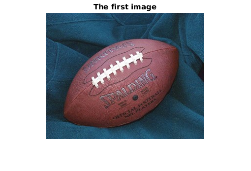
% Open a couple of images.
img1 = imread('football.jpg');
img2 = imread('coins.png');

% Display the first image.
imshow(img1)
title('The first image'); % A title is nice

Figure 2: Original football image.

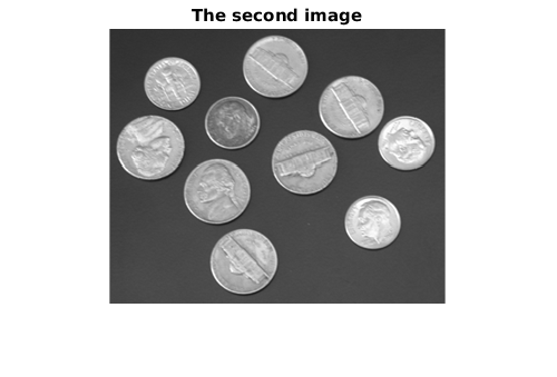
% Display the second image in a new figure.
figure, imshow(img2)
title('The second image');

Figure 3: Original coins image.

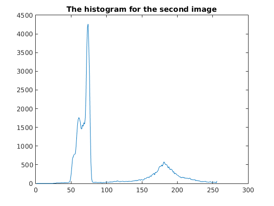
% Histogram the image intensity values.
H = imhist(img2);
plot(H)
title('The histogram for the second image');

Figure 4: Histogram of graylevel values in coins image.

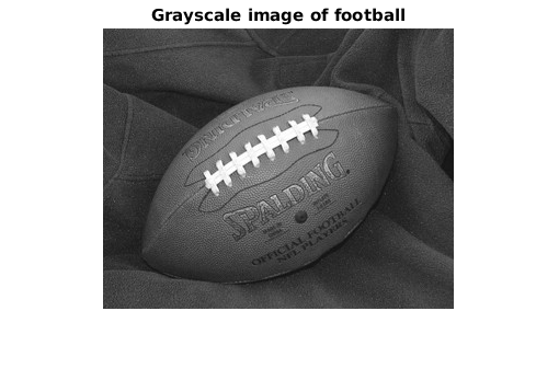
% Converting a colour image with 3 colour channels to a greyscale image
% (the Y in the YIQ colour model).
img1 = imread('football.jpg');
img3 = rgb2gray(img1);
figure, imshow(img3)
title('Grayscale image of football');

Figure 5: Grayscale football image.

Some basic filtering in the image domain.

Now we have jumped into the curriculum of INF2310. You don’t remember, or don’t know?! Don’t hesitate to ask or read up on last courses materials available at http://www.uio.no/studier/emner/matnat/ifi/INF2310/v15/

2D correlation: FILTER2 2D convolution: CONV2 With IMFILTER you can choose either 2D correlation (default) and 2D convolution, and it also has some boundary options.

% Filter IMG3 using a 5x5 mean filter.
h1 = ones(5,5) / 25;
img4 = imfilter(img3,h1); % symmetric filter => correlation = convolution
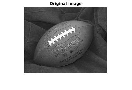
imshow(img3), title('Original image');
figure, imshow(img4), title('Filtered image')

Figure 6: Graylevel football image.

Figure 7: Blurred football obtained using convolution with blurring filter.

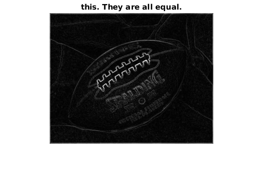
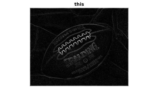
% Find the gradient magnitude of IMG3.
h2x = [-1 -2 -1 ;  0  0  0 ;  1  2  1] % Lack of trailing semicolon will
h2y = [-1  0  1 ; -2  0  2 ; -1  0  1] % print these values.
resX = conv2(double(img3), h2x); % NOTE: DOUBLE type conversion
resY = conv2(double(img3), h2y);
resXY = sqrt(resX.^2 + resY.^2);

The above snippet will print

h2x = 

  -1  -2  -1
   0   0   0
   1   2   1

h2y = 

  -1   0   1
  -2   0   2
  -1   0   1

% Display the gradient magnitude, but not like this:
figure, imshow(resXY);
title('Not like this');

Figure 8: Wrong.

% because the assumed range of the DOUBLE type is [0,1],
% but e.g. one of these ways:
figure, imshow(resXY, []);

Figure 9: Correct alternative 1.

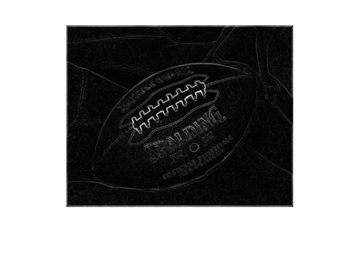
figure, imshow(resXY, [min(resXY(:)) max(resXY(:))]);
title('this')

Figure 10: Correct alternative 2.

figure, imshow(resXY/max(resXY(:)));
title('this or')

Figure 11: Correct alternative 3.

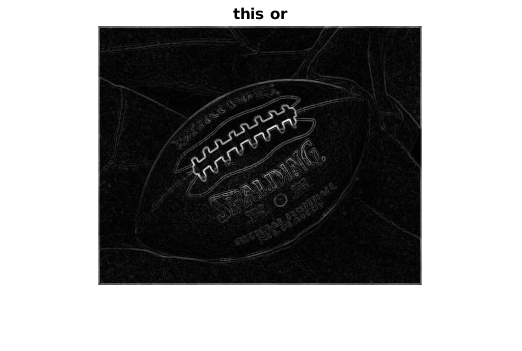
figure, imshow(uint8(resXY/max(resXY(:)).*255));
title('this. They are all equal.');

Figure 12: Correct alternative 4.