Python introduction
This tutorial is a short reference guide and intro to python, focused on image analysis. In this course you can use whatever language you chose, but the examples and solution proposals I create will only be available in python.
There are two main versions of python available: python 2 (v2.7) and python 3 (v3.5), and somewhat inconvenient, python 3 is not always backwards compatible with python 2. This introduction, and solution proposals will assume python 3.5, so if you are religous about keeping to some other version, this is totally okay, but remember that instructions posted here assumes v3.5.
One of the great advantages with python is its large open community, and the wide variety of usefull libraries. As a matter of convenience, I will help you set up an Anaconda virtual environment, and show you how to install relevant packages. With this, whenever you see me importing something in a python script, I should already have described how to get this package. Anaconda is of course optional, but I highly reccomend it.
Table of contents:
Set up python with anaconda
This particular section is written with Linux or Apple Mac in mind, but I am sure that similar things will also work for Windows users.
Python should be included on MacOS, and on most Linux distributions, but for the anaconda version, follow the install instructions at the anaconda site, and verify that anaconda is installed properly. This should be straight forward, and there is no need for me to copy these instructions here.
Create a virtual environment
When working on different projects, it is enormously practical to isolate the different packages you use for the different projects. System-wide installations, with different projects needing different versions of certain packages is a real pain. A virtual environment is a way to isolate a project, such that no conflicts will occur. Below follows a guide on how to create it, but for an external reference, see e.g. here.
Ensure that conda is up to date, and create a virtual environment (this is for python 3.5, but the same is valid for v2.7).
<my_prompt> → conda update conda
<my_prompt> → conda --version
conda 4.3.7
<my_prompt> → conda create -n inf2310 python=3.5 anaconda
where inf2310 is whatever name you want (but preferably something meaningful,
like inf2310). The anaconda argument at the end is optional, but with it, it
installs many useful (and some not so useful) packages.
That is it. You will find the environment located at
/path/to/my/anaconda_folder/envs/inf2310
which in my case is
/home/oskrede/anaconda3/envs/inf2310
To enter this environment, type
<my_prompt> → source activate inf2310
and to exit, type
<my_prompt> → source deactivate
in the command line (from wherever, i.e. you do not need to be located in any particular folder).
When you are in the virtual environment, your command line prompt will look like this
(inf2310) <my_prompt> →
and when you enter python, it will be something like this (print python and hit
return, type exit() to exit)
(inf2310) <my_prompt> → python
Python 3.5.2 |Anaconda 4.2.0 (64-bit)| (default, Jul  2 2016, 17:53:06)
[GCC 4.4.7 20120313 (Red Hat 4.4.7-1)] on linux
Type "help", "copyright", "credits" or "license" for more information.
>>> exit()
(inf2310) <my_prompt> →
Python
Python is a widely used high-level, general-purpose, interpreted, dynamic programming language. Its design philosophy emphasizes code readability, and its syntax allows programmers to express concepts in fewer lines of code than possible in languages such as C++ or Java. The language provides constructs intended to enable clear programs on both a small and large scale.
Python supports multiple programming paradigms, including object-oriented, imperative and functional programming or procedural styles. It features a dynamic type system and automatic memory management and has a large and comprehensive standard library.
-wikipedia
This part is loosely based on excerpts from the more comprehensive python 3 tutorial, and I will try to not go into too much detail. Code blocs will assume that you are in the regular python interpreter:
(inf2310) <my_prompt> → python
Python 3.5.2 |Anaconda 4.2.0 (64-bit)| (default, Jul  2 2016, 17:53:06)
[GCC 4.4.7 20120313 (Red Hat 4.4.7-1)] on linux
Type "help", "copyright", "credits" or "license" for more information.
>>> 2 + 2
4
>>>
or in a text editor, but more on that later.
Types and containers
Python has all available types like int, float, bool and string as you
would expect from any programming language, and they are often implicitly understood
by context (use with care).
Scalar numbers and booleans
>>> some_int = 8
>>> some_float = 8.0
>>> type(some_int)  # prints "<class 'int'>"
>>> type(some_float)  # prints "<class 'float'>"
>>> is_equal = some_int == some_float
>>> type(is_equal)  # prints "<class 'bool'>"
>>> is_equal
True
>>> some_other_int = 4
>>> is_equal = some_int == some_other_int
>>> is_equal
False
>>> t = True
>>> f = False
>>> t and f  # Logical AND
False
>>> t or f   # Logical OR
True
>>> not t    # Logical NOT
False
>>> t != f   # Logical XOR
True
Strings
>>> some_string = 'This is a string'
>>> some_other_string = "This is also a string"
>>> type(some_string)  # prints "<class 'str'>"
>>> type(some_other_string)  # prints "<class 'str'>"
>>> some_string == some_other_string
False
>>> some_other_string = "This is a string"
>>> some_string == some_other_string
True
Lists
Lists are containers, which values are wrapped by square brackets and separated
by commas. They can be sliced, and accesed by their index (note that python is
zero-indexed, and that the slice intervals are from start_index (inclusive)
to end_index (exclusive)).
>>> some_list = [2, 3, 5, 7, 11]
>>> type(some_list)  # prints "<class 'list'>"
>>> some_list[0]
2
>>> some_list[4]
11
>>> some_list[-1]
11
>>> some_list[0:2]
[2, 3]
>>> some_list[:2]
[2, 3]
>>> some_list[3:5]
[7, 11]
>>> some_list[3:]
[7, 11]
>>> some_list[3:-1]
[7]
>>> some_list[1:5]
[3, 5, 7, 11]
>>> some_list[1:5:1]
[3, 5, 7, 11]
>>> some_list[1:5:2]
[3, 7]
>>> some_list[1:5:3]
[3, 11]
>>> some_other_list = [13, 17, 19, 23]
>>> some_list + some_other_list  # List concatenation
[2, 3, 5, 7, 11, 13, 17, 19, 23]
>>> str_list = ['This ', 'is ', 'a ', 'string']
>>> str_list + some_list
['This ', 'is ', 'a ', 'string', 2, 3, 5, 7, 11]
>>> some_list[2] = 1212  # Replace value at index 2 (lists are mutable)
>>> some_list
[2, 3, 1212, 7, 11]
>>> new_list = []  # Initialize empty list
>>> new_list.append(4) # Append to end of list
>>> new_list.append(8)
>>> new_list.append(2)
>>> new_list
[4, 8, 2]
>>> new_list.pop() # Remove last element and return it
2
>>> new_list.remove(8) # Remove element identified by value
>>> new_list
[4]
Dictionaries
Dictionaries are containers which elements can be accessed by keywords, and they have no internal order (you can however sort them by both keywords and values, but I will not go into that here). They are wrapped by curly brackets, key and value pairs are joined by a colon, and separated by commas.
>>> some_dict = {'key1':2, 'key2':'three', 5:'five'}
>>> type(some_dict)  # prints "<class 'dict'>"
>>> some_dict.keys()
dict_keys(['key1', 'key2', 5])
>>> some_dict.values()
dict_values([2, 'three', 'five'])
>>> some_dict['key1']
2
>>> some_dict['key2']
'three'
>>> some_dict[5]
'five'
>>> some_dict['new_key'] = 88  # Adding a new value to a new key
>>> some_dict['new_key']
88
>>> some_dict['key2'] = 88  # Replacing a value for an existing key
>>> some_dict['key2']
88
>>> some_other_dict = {} # Empty initialization
>>> some_other_dict['key'] = 'value' # Everything is as expected
>>> some_other_dict
{'key': 'value'}
Basic operations
Scalar numbers
Nothing out of the ordinary here, the basic binary operations works intuitively.
>>> 2 + 2
4
>>> 2 + 3*4
14
>>> (2 + 3)*4
20
>>> 13 / 5   # Floating point division (integer division in python 2)
2.6
>>> 13 // 5  # Integer division (the quotient in Euclidean division)
2
>>> 13 % 5   # Modulo operator (the remainder in Euclidean division)
3
>>> (13 // 5)*5 + (13 % 5) # Check
13
>>> 2**8  # '**' is the power operator
256
>>> a = 3
>>> a += 3  # Increment by 3
>>> a
6
>>> a -= 2  # Decrement by 2
>>> a
4
>>> a *= 3  # Multiply itself by 3
>>> a
12
>>> a /= 4  # Divide itself by 4 (implicit cast to float)
>>> a
3.0
>>> # a++, a-- and the likes does not exist
Strings and lists
We can also use some handy operations on strings
>>> 'This ' + 'is ' + 'a ' + 'string'  # String concatenation
'This is a string'
>>> str1 = 'This '
>>> str2 = 'is '
>>> str3 = 'a '
>>> str4 = 'string'
>>> str5 = str1 + str2 + str3 + str4
>>> str5
'This is a string'
>>> str1*3 + str2 + str3 + str4
'This This This is a string'
>>> list(str5)  # String to list of characters
['T', 'h', 'i', 's', ' ', 'i', 's', ' ', 'a', ' ', 's', 't', 'r', 'i', 'n', 'g']
>>> word_list = str5.split()  # String to list of words separated by ' ' (whitespace is default)
>>> word_list
['This', 'is', 'a', 'string']
>>> str5.split('i')  # String to list of words separated by 'i'
['Th', 's ', 's a str', 'ng']
>>> ''.join(word_list)  # List to string
'Thisisastring'
>>> ' '.join(word_list) # List to string separated by whitespace
'This is a string'
>>> '_'.join(word_list) # List to string separated by underscore
'This_is_a_string'
>>> str5[8]  # Access element
'a'
>>> str5[8:12]  # Slicing
'a st'
>>> str5[8] = 'some'  # Strings are immutable
Traceback (most recent call last):
File "<stdin>", line 1, in <module>
TypeError: 'str' object does not support item assignment
>>> str5.replace('a string', 'the way to do it')  # But this is allowed
'This is the way to do it'
>>> 'string' in str5  # Check if 'string' is contained in str5
True
>>> 'blablabla' in str5
False
>>> some_list = [2, 3, 5, 7, 11]
>>> 5 in some_list  # This works also for lists
True
>>> some_dict = {1:2, 3:4, 5:6}
>>> 3 in some_dict  # and dictionaries (but defaults to keys)
True
>>> 4 in some_dict
False
>>> 4 in some_dict.values()
True
String formatting
Python string formatting is divided into an old style and a new style, I will cover some of the basics of the new style, but see more at this nice page.
>>> 'One {0}, and another {1}'.format('here', 'one here')  # Explicit placement
'One here, and another one here'
>>> 'One {1}, and another {0}'.format('here', 'one here')  # Reversed order
'One one here, and another here'
>>> 'One {}, and another {}'.format('here', 'one here')  # Implicit order
'One here, and another one here'
>>> '{0:<20} 20 places, and right alignment {1:>20}'.format('Left alignment', '20 places')
'Left alignment       20 places, and right alignment            20 places'
>>> 'Three decimal places (with rounding): {0:.3f}'.format(3.14159265)
'Three decimal places (with rounding): 3.142'
>>> 'Scientific notation: {0:.3e}'.format(0.000314159265)
'Scientific notation: 3.142e-04'
>>> 'Combo: {0:>10,.3f}'.format(3.14159265)
'Combo:      3.142'
Printing
In python 3.x, print is a function that formats
the input and writes to stdout, and this is actually some of the more visible
differences between python 2 and 3.
String formatting in python
>>> print('Hello world')
Hello world
>>> print('Hello', 'world')
Hello world
>>> print('Hello', 'world', 1, 2.3)
Hello world 1 2.3
Scripting
Up until now, we have been using the built in python interpreter, which is
great for testing small commands, and using python as a calculator, but for
more complex programs, it is simply better to script whatever you want in
your favourite editor, and execute it with python. All commads are similar,
but for code snippets, I use >>> to explicitly signal that I am in the
command line interpreter.
Simply open a text editor (vi, emacs, atom, gedit etc.), write some lines
a = 3
b = 4
c = a + b

print(c)
save it as something ending with .py, e.g. test_script.py and run it.
(inf2310) <my_prompt> → python test_script.py
7
You can easily define functions with the def keyword, followed by the name of
the function, and ending with a colon. You must indent all lines that follows
it if you want them in the function, this is how python handles blocks. Remember
to put the function definition above the statements using it. If you want the
function to return something, you use the ‘return’ keyword.
def add_these(x, y):
  z = x + y
  return z

a = 3
b = 4
c = add_these(a, b)

print(c)  # This will print 7
We have not touched upon compund statements yet, but they are easily available (remember the note about indentation above).
some_list = [1, 2, 3, 4, 5, 4, 3, 2, 1]

# Use i to iterate the list values.
for i in some_list:
  if i > 4:
    print(i)

# Use i to iterate the list indices.
for i in range(9):
  if some_list[i] > 4:
    print(i)
Executing it yields
(inf2310) <my_prompt> → python test_script.py
5
4
NumPy
NumPy is the fundamental package for scientific computing with Python. It contains among other things:
- a powerful N-dimensional array object
- sophisticated (broadcasting) functions
- tools for integrating C/C++ and Fortran code
- useful linear algebra, Fourier transform, and random number capabilities
Besides its obvious scientific uses, NumPy can also be used as an efficient multi-dimensional container of generic data. Arbitrary data-types can be defined. This allows NumPy to seamlessly and speedily integrate with a wide variety of databases.
Whenever we are going to do some math on larger arrays (which is almost all the time), we will use numpy. If you are already familiar with matlab, you can check out this tutorial. Numpy should already be installed with the anaconda environment we created above, to be sure, type the following in the command line, and you should see something like this
(inf2310) <my_prompt> → python -c "import numpy as np; print(np.__version__)"
1.11.1
Arrays
A numpy array is a list of values of the same data type. It can be multi-dimensional, and the number of elements in each dimension is given by its shape. One can initialize a numpy array by a nested list.
>>> import numpy as np
>>> a = np.array([[1, 2, 3], [4, 5, 6]])  # Create a 2x3 matrix of ints
>>> print(a)
[[1 2 3]
 [4 5 6]]
>>> a.shape
(2, 3)
>>> type(a)  # prints <class 'numpy.ndarray'>
>>> a.dtype  # Should be 'int64', i.e. 64 bits signed integer
dtype('int64')
>>> at = a.T # Transpose
>>> print(at)
[[1 4]
 [2 5]
 [3 6]]
>>> b = np.array([[1, 2, 3], [3, 2, 1]])
>>> print(a + b)     # Element-wise addition
[[2 4 6]
 [7 7 7]]
>>> print(a * b)     # Element-wise multiplication
[[ 1  4  9]
 [12 10  6]]
>>> c = b.dot(at)    # Matrix multiplication
>>> print(c)
[[14 32]
 [10 28]]
>>> np.linalg.inv(c) # Matrix inverse (note that it lies in numpy linalg)
array([[ 0.38888889, -0.44444444],
       [-0.13888889,  0.19444444]])
You can also initialize numpy arrays with some existing ones
>>> import numpy as np
>>> a = np.zeros((2, 3))  # 2x3 array filled with zeros of 64 bit signed floats
>>> print(a)
[[ 0. 0. 0.]
 [ 0. 0. 0.]]
>>> print(a.dtype)
float64
>>> b = np.ones((2, 3))  # 2x3 array filled with ones of 64 bit signed floats
>>> print(b)
[[ 1. 1. 1.]
 [ 1. 1. 1.]]
>>> c = np.eye(3) # 3x3 identity matrix of 64 bit signed floats
>>> print(b)
[[ 1. 0. 0.]
 [ 0. 1. 0.]
 [ 0. 0. 1.]]
>>> d = np.random.random((2, 3))  # 2x3 array filled with values in Unif(0, 1)
>>> print(d)
[[ 0.83841548  0.94643209  0.83842389]
 [ 0.0357995   0.95270445  0.49803594]]
We can slice and access arrays like with normal python lists, and some more.
>>> import numpy with np
>>> a = np.array([[1, 2, 3], [4, 5, 6]])
>>> print(a[1, 2])
6
>>> print(a[:, 2]) # Note that the result is a 1 dimensional array (no distinction between row and column vector)
[3 6]
>>> b = a > 2  # Boolean array
>>> print(b)
[[False False  True]
 [ True  True  True]]
>>> a[b] = 9  # Use this to set all elements larger than 2 to 9
>>> print(a)
[[1 2 9]
 [9 9 9]]
For more fun with numpy, see the numpy reference documentation.
SciPy
Scipy is a collection of open source software tools for scientific computing in Python. Its domain reach over libraries such as NumPy and Matplotlib (more about that later), so a comprehensive guide is far beyond the scope of this simple introduction. If you followed the anaconda installation above, scipy should already be installed, and you can read more about it in the SciPy documentation.
I will occationally use functions defined in the scipy library, as they have many great tools for linear algebra, signal processing, fourier transforms, and image analysis (to name a few).
OpenCV
To help us with the image processing and analysis, I choose to show openCV, as it is a great tool for computer vision. From its own front page
It has C++, C, Python and Java interfaces and supports Windows, Linux, Mac OS, iOS and Android. OpenCV was designed for computational efficiency and with a strong focus on real-time applications. Written in optimized C/C++, the library can take advantage of multi-core processing. Enabled with OpenCL, it can take advantage of the hardware acceleration of the underlying heterogeneous compute platform.
Many of the tools provided by openCV is also available in SciPy, and for this class, it is probably sufficient with only one of them. I think, however, that it is valuable to familiarize oneself with both tools, especially if you are to apply image analysis beyond this course in the future.
Installation
We use the conda package manager to install it (be careful that it is compatible with your python version).
Be sure to be in the newly created conda environment, and check that openCV is not already installed.
<my_prompt> → source activate inf2310
(inf2310) <my_prompt> → python -c "import cv2"
Traceback (most recent call last):
  File "<string>", line 1, in <module>
ImportError: No module named 'cv2'
Install OpenCV and print its version. You will be asked to confirm your installation, if you want
to continue, you press y.
NB! This part was updated 08.02.2017, as I received some feedback from students not able to install OpenCV with the previous instructions. Hopefully, this will work for everybody, but if you are experiencing trouble (and is participating in the inf2310 course), please contact me, and I will try to help you out. Also note that it is not very important to install OpenCV for this course, we work on a very fundamental level, so there will always be other packages that we can use (e.g. scikit-image, which we may use sometimes anyway).
(inf2310) <my_prompt> → conda install -c conda-forge opencv=3.1.0
Fetching package metadata ...........
Solving package specifications: .

Package plan for installation in environment /home/icgi-tf/anaconda3/envs/inf2310:

The following NEW packages will be INSTALLED:

opencv: 3.1.0-np111py35_1 conda-forge

Proceed ([y]/n)? y

opencv-3.1.0-n 100%
|#############################################################################| Time: 0:00:31   1.19 MB/s


(inf2310) <my_prompt> → python -c "import cv2; print(cv2.__version__)"
3.1.0
(If this do not work either, you can try to remove opencv, and install from another channel:
<my_prompt> → conda remove opencv
<my_prompt> → conda update conda
<my_prompt> → conda install -c menpo opencv3=3.2.0
)
Matplotlib
Matplotlib is a plotting library, which module
matplotlib.pyplot provides plotting functions similar to that of matlab.
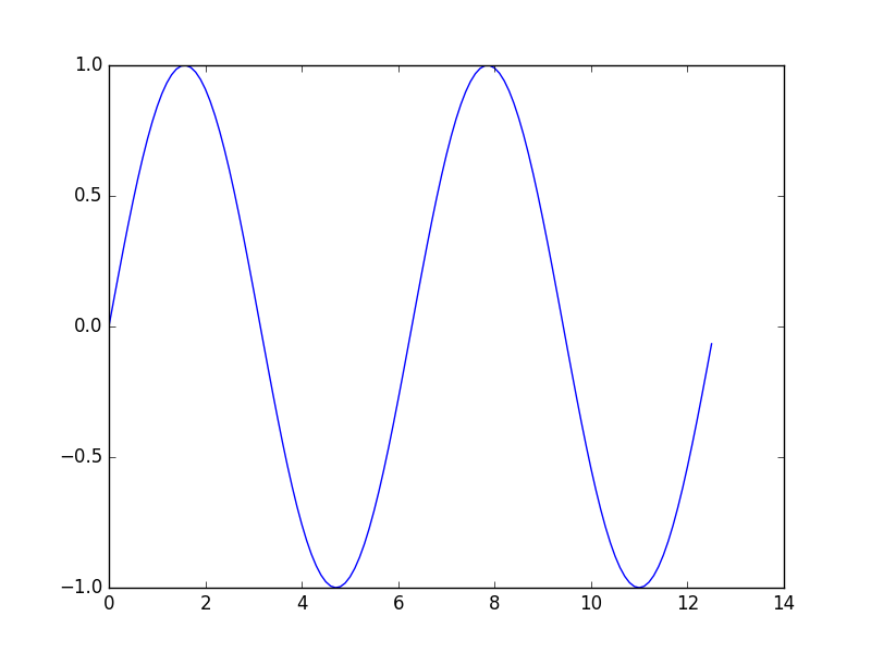
For a simple 2D plot
import numpy as np
import matplotlib.pyplot as plt

# Create some points following a sine curve
x = np.arange(0, 4*np.pi, 0.1)
y = np.sin(x)

# Plot the points, and remember to call plt.show() at the end
plt.plot(x, y)
plt.show()
This should produce something like this
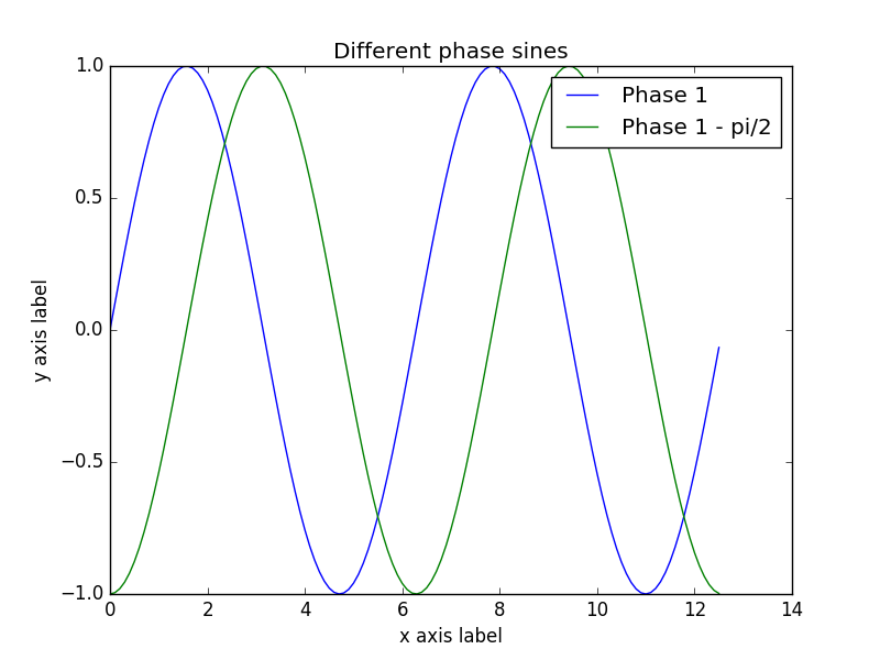
For a simple 2D plot with multiple graphs
import numpy as np
import matplotlib.pyplot as plt

# Create some points following sine curves with different phase
x = np.arange(0, 4*np.pi, 0.1)
y_1 = np.sin(x)
y_2 = np.sin(x - np.pi/2)

# Plot them
plt.plot(x, y_1)
plt.plot(x, y_2)
plt.xlabel('x axis label')
plt.ylabel('y axis label')
plt.title('Different phase sines')
plt.legend(['Phase 1', 'Phase 1 - pi/2'])
plt.show()
which should look like this
We can also specify multiple figures, which should result in different plot windows.
import numpy as np
import matplotlib.pyplot as plt

# Create some points following sine curves with different phase
x = np.arange(0, 4*np.pi, 0.1)
y_1 = np.sin(x)
y_2 = np.sin(x - np.pi/2)

# First
plt.figure(0)
plt.plot(x, y_1)

# Second
plt.figure(1)
plt.plot(x, y_2)

plt.show()
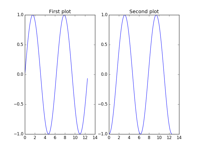
You can also get different plot graphs in the same figure
import numpy as np
import matplotlib.pyplot as plt

# Create some points following sine curves with different phase
x = np.arange(0, 4*np.pi, 0.1)
y_1 = np.sin(x)
y_2 = np.sin(x - np.pi/2)

# Create a subplot with height 1 and with 2 (meaning that you will have 2
# plots side by side), and specify that this is the first.
plt.subplot(1, 2, 1)
plt.plot(x, y_1)
plt.title('First plot')

# Specify the second one
plt.subplot(1, 2, 2)
plt.plot(x, y_2)
plt.title('Second plot')

plt.show()
Images
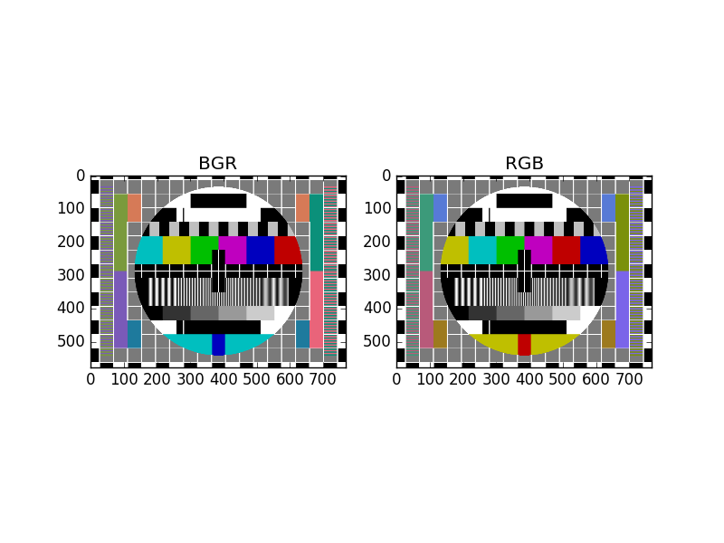
For images, we will use openCV to read, manipulate, and write them, but use pyplot to plot them (even though openCV also provides this functionality).
import numpy as np
import matplotlib.pyplot as plt
import cv2
imagefile = './assets/images/test_image.png' # Change this to something useful
# Read image as bgr color image (which is simply a rank 3 numpy array with shape
# (num_height_pixels x num_width_pixels x num_channels))
bgr_image = cv2.imread(imagefile, cv2.IMREAD_COLOR)
print('Color image info:')
print('Type: ', type(bgr_image))
print('Data type: ', bgr_image.dtype)
print('Shape: ', bgr_image.shape)
print('Min val: ', np.min(bgr_image), '. Max val: ', np.max(bgr_image))
# Transform to rgb and plot both
blue, green, red = cv2.split(bgr_image)
rgb_image = cv2.merge([red, green, blue])
# Note that the same could be achieved with the colorspace conversion function cvtColor:
# rgb_image = cv2.cvtColor(bgr_image, cv2.COLOR_BGR2RGB)
plt.figure(0)
plt.subplot(1, 2, 1)
plt.imshow(bgr_image)
plt.title('BGR')
plt.subplot(1, 2, 2)
plt.imshow(rgb_image)
plt.title('RGB')
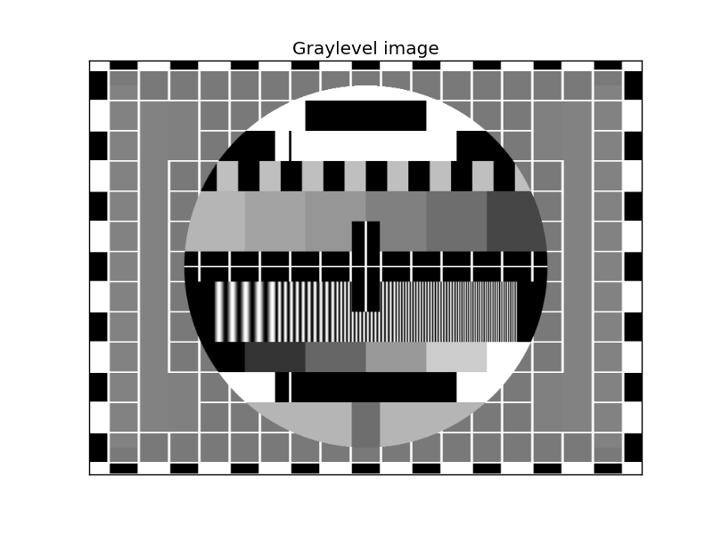
# Read the same image in as a graylevel image, and plot it
gray_image = cv2.imread(imagefile, cv2.IMREAD_GRAYSCALE)
# As before, we could have used colorspace conversion for the same result
# gray_image = cv2.cvtColor(bgr_image, cv2.COLOR_BGR2GRAY)
# gray_image = cv2.cvtColor(rgb_image, cv2.COLOR_RGB2GRAY)
print('Graylevel image info:')
print('Type: ', type(gray_image))
print('Data type: ', gray_image.dtype)
print('Shape: ', gray_image.shape)
print('Min val: ', np.min(gray_image), '. Max val: ', np.max(gray_image))
plt.figure(1)
plt.imshow(gray_image, cmap='gray') # Note the colormap definition
plt.xticks([]) # Remove ticks on x axis
plt.yticks([]) # Remove ticks on y axis
plt.title('Graylevel image')
plt.show()
This will print
Color image info:
Type:  <class 'numpy.ndarray'>
Data type:  uint8
Shape:  (576, 768, 3)
Min val:  0 . Max val:  255
Graylevel image info:
Type:  <class 'numpy.ndarray'>
Data type:  uint8
Shape:  (576, 768)
Min val:  0 . Max val:  255
provided that you read in the test_image.png from assets, the
plots will look like this.