Solution proposal - week 2
Automatically generated from this jupyter notebook.
Solution to python exersices, inf2310, week 2
Task 1
Import the necessary libraries
%matplotlib inline

import cv2
import numpy as np
import matplotlib.pyplot as plt
Load and display the mona lisa image
image = cv2.imread('../../assets/images/mona.png', cv2.IMREAD_GRAYSCALE)
plt.imshow(image, cmap='gray')
<matplotlib.image.AxesImage at 0x7f4efe60cac8>
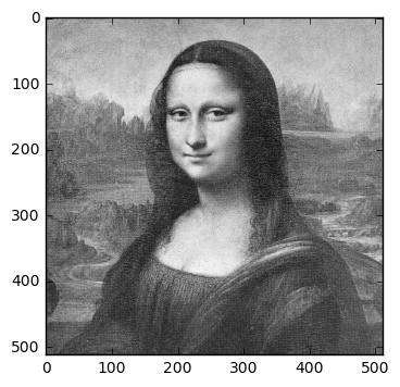
Let us print some properties with the image, like the shape, the data type and the size.
print(image.shape)
print(image.dtype)
(512, 512)
uint8
The type uint8 is a common data type for images, and it means that each value in the image is stored as an unsigned 8-bit value. This means that the smallest value is 0 and the greatest value is 255, since
1 byte is 8 bits, so we could find the number of bytes the image occupies by multiplying the number of pixels in the image with 1 byte.
print(512 * 512 / 1024) # Result in KiB (Kibibyte)
256.0
Let us test this by measuring the size of the image object (notice that there is some overhed in python objects, so this is really not very reliable).
import sys
print(sys.getsizeof(image) / 1024)
256.109375
Okay, this was a bit (…) out of the purpouse of the task, let us get back to the actual matters in hand. Now, we initialize the resulting image, and populate it.
M, N = image.shape
diff_image = np.zeros((M, N), dtype='uint8') # Default type is 'float64'
for i in range(1, M): # From (including) to (not including) M
    for j in range(N): # Implicit from 0 to (not including) N
        diff_image[i, j] = image[i, j] - image[i - 1, j]
/home/oskrede/anaconda3/envs/inf2310/lib/python3.5/site-packages/ipykernel/__main__.py:5: RuntimeWarning: overflow encountered in ubyte_scalars
This prints a warning on type overflow, since it is trying to assigning negative values to a uint8 array. Fix this by adding a bias of e.g. 128
for i in range(1, M): # From (including) to (not including) M
    for j in range(N): # Implicit from 0 to (not including) N
        diff_image[i, j] = 128 + image[i, j] - image[i - 1, j]
Plot the result
plt.imshow(diff_image, cmap='gray')
<matplotlib.image.AxesImage at 0x7f4efe6c2438>
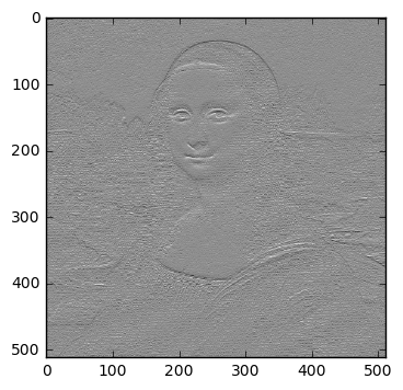
As you should expect, we get dark values at edges going from bright to dark values in the positive vertical direction. Similarly , we get bright values at edges going from dark values to bright values in the positive vertical direction.
Let us now try to scale the result image with a scalar greater than 1. We also change the datatype of image and diff_image to int (32-bit signed integer) to not get overflow warnings.
c = 2.5
image = image.astype('int')
diff_image = diff_image.astype('int')
for i in range(1, M): # From (including) to (not including) M
    for j in range(N): # Implicit from 0 to (not including) N
        diff_image[i, j] = 128 + c*(image[i, j] - image[i - 1, j])
plt.imshow(diff_image, cmap='gray')
<matplotlib.image.AxesImage at 0x7f4efe7aa6a0>
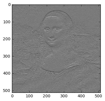
The result is that the contrast increases (as we might expect).
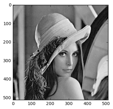
Task 4
Load and display the image, we will also display the number of unique values in the image.
image = cv2.imread('../../assets/images/lena.png', cv2.IMREAD_GRAYSCALE)
plt.imshow(image, cmap='gray')
print('Number of unique values: ', len(np.unique(image)))
Number of unique values: 216

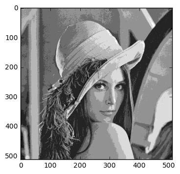
Now, let us requantize the image, and display the effect. First, we try with 1 fewer bit.
bit = 7
requantized_image = (image / (2**(8 - bit))).astype('uint8')
plt.imshow(requantized_image, cmap='gray')
print('Number of unique values: ', len(np.unique(requantized_image)))
Number of unique values: 110

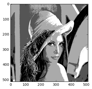
bit = 6
requantized_image = (image / (2**(8 - bit))).astype('uint8')
plt.imshow(requantized_image, cmap='gray')
print('Number of unique values: ', len(np.unique(requantized_image)))
Number of unique values: 56

bit = 5
requantized_image = (image / (2**(8 - bit))).astype('uint8')
plt.imshow(requantized_image, cmap='gray')
print('Number of unique values: ', len(np.unique(requantized_image)))
Number of unique values: 28
bit = 4
requantized_image = (image / (2**(8 - bit))).astype('uint8')
plt.imshow(requantized_image, cmap='gray')
print('Number of unique values: ', len(np.unique(requantized_image)))
Number of unique values: 15

bit = 3
requantized_image = (image / (2**(8 - bit))).astype('uint8')
plt.imshow(requantized_image, cmap='gray')
print('Number of unique values: ', len(np.unique(requantized_image)))
Number of unique values: 8
bit = 2
requantized_image = (image / (2**(8 - bit))).astype('uint8')
plt.imshow(requantized_image, cmap='gray')
print('Number of unique values: ', len(np.unique(requantized_image)))
Number of unique values: 4
bit = 1
requantized_image = (image / (2**(8 - bit))).astype('uint8')
plt.imshow(requantized_image, cmap='gray')
print('Number of unique values: ', len(np.unique(requantized_image)))
Number of unique values: 2
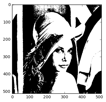
As we can see, we ended up with a binary version of our original image. However, we also see that we could manage with only 5 bits, and still have a quite good visual impression of the image.