Exercise 5 - Object description

Task 1

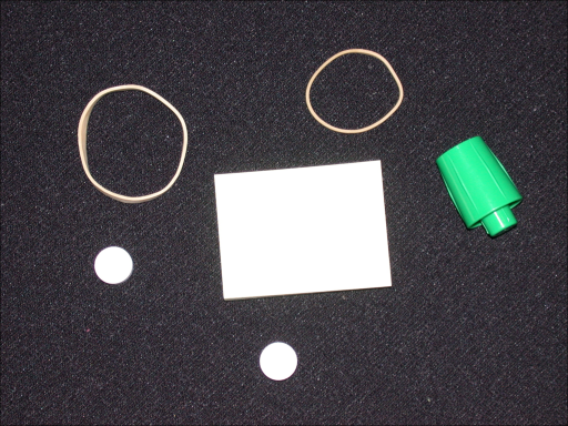
Recognition of round objects in an image using python. The image we will be looking at is called pillsetc.png, and can be found in the image folder.

Figure 1: Image 'pillsetc.png'.

Step 1: Read image

Read the image.

import numpy as np
import cv2
  
# Substitute this with your location
image_file = '../../images/pillsetc.png'
# OpenCV reads color images as BGR instead of RGB
rgb_image = cv2.cvtColor(cv2.imread(image_file, cv2.IMREAD_COLOR), cv2.COLOR_BGR2RGB)

Step 2: Threshold the image

Convert the image to a binary black and white image with Otsu thresholding.

gray_image = cv2.cvtColor(rgb_image, cv2.COLOR_RGB2GRAY)
threshold, thresh_image = cv2.threshold(gray_image, 0, 255, cv2.THRESH_BINARY+cv2.THRESH_OTSU)

Step 3: Remove the noise

Using morphology functions, remove pixels which do not belong to the objects of interest.

from skimage import morphology
from scipy.ndimage.morphology import binary_fill_holes

# Remove objects containing fewer than 30 pixels (both gives essentially the
# same output)
rmnoise_image = morphology.remove_small_objects(thresh_image.astype(bool), min_size=30)
#rmnoise_image = morphology.binary_opening(thresh_image)

# Fill a gap in the cap of the pen
fillcap_image = morphology.binary_closing(rmnoise_image, selem=morphology.disk(2))

# Fill holes
clean_image = binary_fill_holes(fillcap_image)

Step 4: Find the boundaries

Find the boundaries of the objects in the image with the function cv2.findContours. We will only search for external boundaries, that is, no inner boundaries, or boundaries in enclaves (making the filling of the holes in the previous step redundant, but nevermind), we achieve this with option cv2.RETR_EXTERNAL. We also chose to find all contour points, and use option cv2.CHAIN_APPROX_NONE for this.

See more here and here.

But note that these refer to OpenCV 2, and have been changed in OpenCV 3, see more here and here.

The most visible change is that in version 2 it is

contours, hierarchy = cv2.findContours(...)

contrary to version 3 which is

label_image, contours,  hierarchy = cv2.findContours(...)

_, contours, _ = cv2.findContours(clean_image.astype(np.uint8), # pylint: disable=unused-variable
                                  cv2.RETR_EXTERNAL,
                                  cv2.CHAIN_APPROX_NONE)

# Draw the contours and the objects they enclose
obj_image = np.zeros(clean_image.shape)
for ind, cnt in enumerate(contours):
  col = 255 * (ind + 1) / len(contours) # Different colors, to differentiate objects
  cv2.drawContours(obj_image, [cnt], 0, col, -1)

Step 5: Determine which objects are round

For a circle with area $A$ and circumference $C$ , the following relationship will hold

$\frac{4 \pi A}{C^2} = 1.$

Therefore, for an object with area $A$ and perimeter $P$ , we use the metric $\alpha = \frac{4 \pi A}{P^2}$ to determine how round the shape is, the closer $\alpha$ is to $1$ , the rounder it is. Mark the center of all objects rounder than some threshold $t$ , $\alpha > t$ .

import matplotlib.pyplot as plt

round_thresh = 0.9

plt.figure()
height, width = obj_image.shape
plt.imshow(obj_image.astype(np.uint8), cmap='gray')

print('Object      Area Perimeter Roundness')
for ind, contour in enumerate(contours):
  # Compute a simple estimate of the object perimeter
  # contour is a list of N coordinate points (x_i, y_i), and the perimeter is computed as
  # perimeter = sum_{i=0}^{N-2} ( sqrt( (x_{i+1} - x_i)^2 + (y_{i+1} - y_i)^2 ))
  delta_squared = np.diff(contour, axis=0)*np.diff(contour, axis=0)
  perimeter = np.sum(np.sqrt(np.sum(delta_squared, axis=1)))
  
  # or use the built in arcLength() (both arcLength() and contourArea() are
  # based on Freeman chain codes).
  perimeter = cv2.arcLength(contour, True)

  area = cv2.contourArea(contour)
  alpha = 4*np.pi*area/(perimeter**2)
  print('{0:>6} {1:>9,.0f} {2:>9,.2f} {3:>9,.3f}'.format(ind, area, perimeter, alpha))

  # Plot a red circle on the centroid of the round objects
  if alpha > round_thresh:
    moments = cv2.moments(contour)
    cx = int(moments['m10'] / moments['m00'])
    cy = int(moments['m01'] / moments['m00'])
    plt.plot(cx, cy, 'ro')

# Fit the plt.plot() figures to the plt.imshow()
axes = plt.gca()
axes.set_xlim([0, width])
axes.set_ylim([height, 0])

plt.show()

Task 2

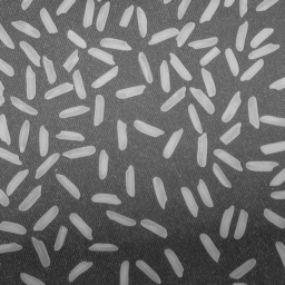
In this task, we will look at the image rice.png (which can be found here ), segment out the grains, and mark the ones with a certain orientation.

Figure 2: Image `rice.png`.

Step 1: Read the image

Read the image rice.png as a graylevel image.

image_file = '../../images/rice.png'
image = cv2.imread(image_file, cv2.IMREAD_GRAYSCALE)

Step 2: Use morphological opening to estimate the background

Notice that the background illumination is brighter in the center of the image than at the bottom.

selem = cv2.getStructuringElement(cv2.MORPH_ELLIPSE, (31, 31))
background = cv2.morphologyEx(image, cv2.MORPH_OPEN, selem)

Step 3: Subtract the background image from the original image

foreground = cv2.subtract(image, background)

Step 4: Increase the image contrast

Increase the image contrast, note that this might not work as expected, since the much of the contrast in the bacground noise is also enhanced.

# Here, we can implement our own, or use the built in global histogram
# equalization
contrasted = cv2.equalizeHist(foreground)
# Or we can try out the Contrast Limited Adaptive Histogram Equalization
#clahe = cv2.createCLAHE()
#contrasted = clahe.apply(foreground)

Step 5: Threshold the image

Create a new binary image by thresholding the contrast adjusted image.

thresh_otsu, binary_image = cv2.threshold(contrasted.astype(np.uint8), 0, 255,
                                          cv2.THRESH_BINARY+cv2.THRESH_OTSU)

Step 6: Label objects in the image

num_labels, label_image = cv2.connectedComponents(binary_image, connectivity=4)

Step 7: Examine the label image

Every pixel in a distinct object (a connected region) is labeled with the same label, we will take a look at the grain labeled 43.

# First, we select the grain labeled 43, and finds its contour
single_grain_full = (label_image == 43)
_, cnt_list, _ = cv2.findContours(single_grain_full.astype(np.uint8),
                                  cv2.RETR_EXTERNAL,
                                  cv2.CHAIN_APPROX_NONE)

# As there is only one contour, we select it, and use it to compute a
# bounding box around the grain
grain_contour = cnt_list[0]
y_start, x_start, dy, dx = cv2.boundingRect(grain_contour)
grain_min_bbox = label_image[x_start:x_start+dx, y_start:y_start+dy].astype(np.uint8)

# grain_min_bbox is the minimal bounding box around the grain, so we pad it a
# bit before we display it.
grain_bbox = cv2.copyMakeBorder(grain_min_bbox, 10, 10, 10, 10,
                                cv2.BORDER_CONSTANT, value=0)
# This grain_bbox is an image of the grain with label 43, and should now have a
# 10 pixel wide black frame around the grain.

Step 8: View the whole label image

View the label image, here you can either use the function label2rgb() from skimage.color, or just use a nice colormap for the graylevel image.

from skimage.color import label2rgb

rgb_label_image = label2rgb(label_image)

Step 9: Measure object properties in the image

For all objects in the label image, compute moments, and from them, the area and centroid of the object. Here I show how you can do it in openCV, but I encourage you to implement your own moments. Given a contour (a list of pixel indices belonging to the boundary of the object), moments = cv2.moments(contour) returns a dictionary of moments, which elements can be accessed like moments['m00'] for the zeroth order moment, and moments['mu20'] for the second order central moment about $x$ .

# moments from contours and greens theorem
_, contour, _ = cv2.findContours(label_image.astype(np.uint8),
                                 cv2.RETR_EXTERNAL,
                                 cv2.CHAIN_APPROX_NONE)
# Put the moments of each contour in a dictionary. Note that we here
# potentially lose the original labeling of the grains.
moment_dict = {}
for ind, cnt in enumerate(contour):
  moment_dict[ind] = cv2.moments(cnt)

We can now compute the area and centroid for each grain by traversing this dictionary.

obj_properties = {}
for ind, obj_moments in moment_dict.items():
  if obj_moments['m00'] > 0: # See why at cv2.moments() documentation
    # Compute properties
    area = obj_moments['m00']
    cx = obj_moments['m10'] / obj_moments['m00']
    cy = obj_moments['m01'] / obj_moments['m00']
    
    # Store properties
    props = {}
    props['area'] = area
    props['cx'] = cx
    props['cy'] = cy

    obj_properties[ind] = props

Step 10: Compute statistics about properties of the objects in the image

areas = []
for ind, props in obj_properties.items():
  areas.append(props['area'])
print('Grain {} has the largest area of {} pixels'.format(np.argmax(areas),
                                                          np.max(areas)))
print('Mean area: ', np.mean(areas))

Step 11: Create a histogram of the area of the grains

plt.figure()
plt.hist(areas, bins=30, normed=False, range=[np.min(areas), np.max(areas)])
plt.show()

Step 12: Measure the orientation of the grains

By computing the central moments of each object, we can obtain the object’s orientation. Extend the code, and repeat Step 9, Step 10 and Step 11, but for the orientation angle.

Step 13: Select grains with a certain orientation angle

Find a way to display the grains with an orientation angle in the range of [-20, 20] degrees.

Task 3

Use the images circle2.png, circle5.png, and circle15.png (which can be found in the image folder), to evaluate the accuracy of the different formulas for estimation of area and perimeter discussed in the lecture slides.

Task 4: Object features - moments (from exam 2013)

a)

How do we define the moments of inertia $I$ , of an object in a gray level image?

b)

In terms of moments of inertia, what is the requirement for a 2D object to exhibit a unique orientation?

c)

Show the simple formulation of the two moments of inertia $I_{20}(p_x, p_y)$ and $I_{20}(p_x, p_y)$ about

its center of mass, $(p_x, p_y) = (c_x, c_y)$ ,
the parallel image coordinate axes, $(p_x, p_y) = (0, 0)$ .