Exercise 9 - Linear transforms

Task 1

You are given data from two classes with means and covariances

$\mu_1 = \left[ \begin{array}{c} 3 \\ 6 \end{array} \right], \quad \Sigma_1 = \left[ \begin{array}{cc} 1/2 & 0 \\ 0 & 2 \end{array} \right], \quad \Sigma_1^{-1} = \left[ \begin{array}{cc} 2 & 0 \\ 0 & 1/2 \end{array} \right],$ $\mu_2 = \left[ \begin{array}{c} 3 \\ -2 \end{array} \right], \quad \Sigma_2 = \left[ \begin{array}{cc} 2 & 0 \\ 0 & 2 \end{array} \right], \quad \Sigma_2^{-1} = \left[ \begin{array}{cc} 1/2 & 0 \\ 0 & 1/2 \end{array} \right].$

a)

Compute the eigenvectors and eigenvalues of the covariance matrices, and use them to sketch the contours of the covariance matrices in a plot.

b)

Show that the desicion boundary $d_1(x) = d_2(x)$ in this case can be expressed as

$x_2 = \frac{3}{16} x_1^2 - \frac{9}{8} x_1 + \frac{59}{16} - \frac{1}{4}\log(2),$

where $x = (x_1, x_2)$ is the feature vector.

c)

Plot the resulting desicion boundary (in e.g. python or matlab).

d)

Create a synthetic image with two bands (channels), with samples that span the entire feature space (e.g. from -10 to 10 for both features). For simplicity, let us consider a course grid of samples on integer values $(-10, -9, \cdots, 10)$ . Feature 1 should look like a horizontal ramp from -10 to 10 (inclusive), and feature 2 like a vertical ramp from -10 to 10 (inclusive).

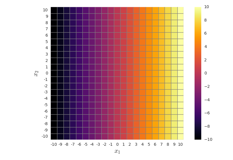
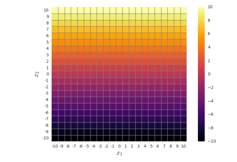
Figure 1.1 Feature image 1 (left) and 2 (right).

This corresponds to creating feature vectors that span the entire feature space (from -10 to 10). If we later classify all these feature vectors, the resulting classification map should have the same decision boundary as the plot we computed in b) and plotted c). This is just a way to create a visualization of the decision boundary without computing it analytically.

e)

Classify the image, and verify that the shape of the decision boundary you got in c) is the same as you get after classifying the image.

Task 2 - Principal component analysis

In this exercise we will implement and explore linear feature transforms for feature extraction for images. As in the other classification exercises, we will work with a 6-band satellite image from Kjeller (tm1.png, …, tm6.png), with training and test masks (tm_train.png, tm_test.png) found here.

Load the images.
Put all the image data into a matrix of shape ( $6, h\times w$ ), where $h$ is the height of the images, $w$ is the width, and we have 6 features. That is, one column for each pixel, where each row correspond to one feature.
Compute the covariance matrix of this data array.
Use a built-in routine to compute the eigenvectors and eigenvalues of the covariance matrix.
Form a matrix $A$ which columns are the eigenvectors of the covariance matrix.
Compute the 6 principal components of the data vector, where the $k$ th component at position $i=1, \cdots, h\times w$ can be computed as the inner product between the feature vector at position $i$ and the $k$ th column of $A$ : $y_{ki} = a_k^\intercal x_i$ .
Reshape the principal component data vector back to a 2D image geometry, that is, a $h\times w$ image for each of the 6 principal components.
Display the different principal component images. Looking at them, how many do you think are useful for classification?
Plot the eigenvalues normalized by the sum of all the eigenvalues.