Task 1 (Problem 10.2 in Gonzalez and Woods)

Task 2 (Problem 10.38 in Gonzalez and Woods)

Task 3 (Problem 10.39 in Gonzalez and Woods)

Task 4 (Problem 10.43 in Gonzalez and Woods)

Task 5 — Python exercise with watershed segmentation.

Step 1 - Create the image

Make a binary image containing two overlapping circular objects (see Figure 1).

import numpy as np

center1 = -10
center2 = -center1
dist = np.sqrt(2*(2*center1)**2)
radius = 1.4*dist/2
lims = (np.floor(center1 - 1.2*radius), np.ceil(center2 + 1.2*radius))
x, y = np.meshgrid(np.arange(lims[0], lims[1]), np.arange(lims[0], lims[1]))
disk1 = np.sqrt((x - center1)**2 + (y - center1)**2) <= radius
disk2 = np.sqrt((x - center2)**2 + (y - center2)**2) <= radius
disks = np.logical_or(disk1, disk2)

Figure 1 Two overlapping disks.

Step 2 - Compute distance transform

Compute the (euclidean) distance transform of the complement of the binary image.

import scipy.ndimage as ndi

dist_trans_img = ndi.distance_transform_edt(disks)

Step 3 - Create markers (not in original exercise)

Create markers to be used as seeds for the watershed at the local maxima in the distance transformed image.

from skimage import feature
local_maxima = feature.peak_local_max(dist_trans_img, indices=False,
                                      footprint=np.ones((3, 3)), labels=disk_img)
markers = ndi.label(local_maxima)[0]

Step 4 - Complement the distance transform

neg_dist_trans_img = -dist_trans_img.astype('float64')

Step 5 - Compute the watershed transform

from skimage import morphology
labels = morphology.watershed(neg_dist_trans_img, markers, mask=disks)

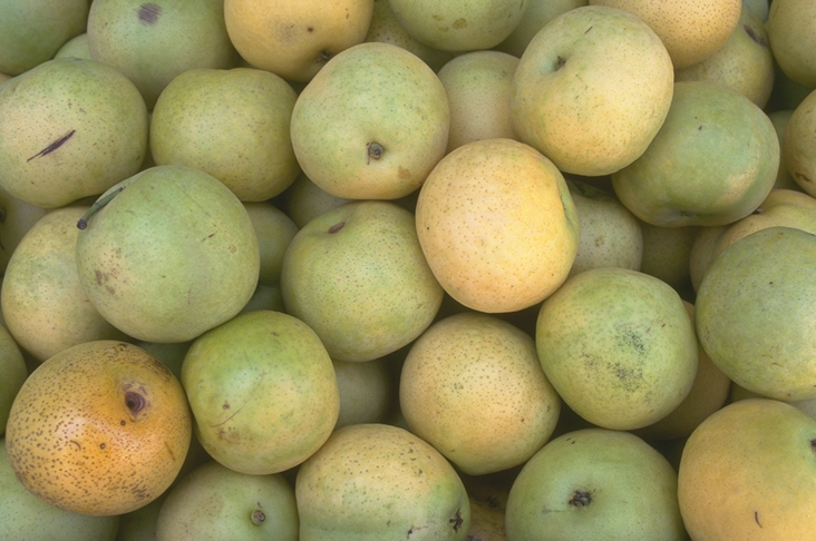
Task 6 — Segmentation of pears using morphology and watershed.

Step 1 - Read the image as a graylevel image

Read in the image pears.png (found here) and convert it to grayscale.

import cv2
image = cv2.imread('../../images/pears.png', cv2.IMREAD_GRAYSCALE)

Figure 2 `pears.png`.

Step 2 - Use gradient magnitude as the segmentation function

Compute the gradient magnitude of the image using Sobel convolution kernels.

sobelx = cv2.Sobel(image, cv2.CV_64F, 1, 0, ksize=3)
sobely = cv2.Sobel(image, cv2.CV_64F, 0, 1, ksize=3)

# Compute gradient magnitude
grad_magn = np.sqrt(sobelx**2 + sobely**2)
# Put it in [0, 255] value range
grad_magn = 255*(grad_magn - np.min(grad_magn)) / (np.max(grad_magn) - np.min(grad_magn))

Can you segment the image by using watershed directly on the gradient magnitude?

Step 3 - Mark the foreground objects

A variety of procedures could be applied here to find the foreground markers, which must connected blobs of pixels inside each of the foreground objects. In this example you’ll use morphological techniques called opening-by-reconstruction and closing-by-reconstruction to clean the image. These operations will create flat maxima inside each object that can be located by some local maxima detector.

Opening is erosion followed by dilation, while opening-by-reconstruction is erosion followed by a morphological reconstruction. Let us compare the two.

First, compute the opening.

selem = morphology.disk(20)
opened = morphology.opening(image, selem)

Next, compute the opening-by-reconstruction. We will first compute the erosion of the image and use this as a seed or a marker image for the reconstruction. The seed specifies the values that are dilated (or eroded in the case of closing-by-reconstruction). Then, we will use original image as a mask, this mask determines the maximum allowed value at each pixel (this is for dilation, and conversly, the mask determines the minimum allowed value at each pixel for erosion).

eroded = morphology.erosion(image, selem)
opening_recon = morphology.reconstruction(seed=eroded, mask=image, method='dilation')

Following the opning with a closing can remove the dark spots and stem marks. Compare a regular morphological closing with a closing-by-reconstruction. First, try to use closing on the opened image.

closed_opening = morph.closing(opened, selem)

Now, use reconstruct the dilated version of the image generated by opening-by-reconstruction. Notice that we do not need to use the complement in the input here (as we do in matlab), but rather set method='erosion' in stead.

dilated_recon_dilation = morph.dilation(opening_recon, selem)
recon_erosion_recon_dilation = morph.reconstruction(dilated_recon_dilation,
                                                    opening_recon,
                                                    method='erosion').astype(np.uint8)

As a side-note, if you want to compute the equivalent with opening-by-reconstruction in stead of closing-by-reconstruction as we used, you can do it. First we will need an imcomplement(...) function.

def imcomplement(image):
  """Equivalent to matlabs imcomplement function"""
  min_type_val = np.iinfo(image.dtype).min
  max_type_val = np.iinfo(image.dtype).max
  return min_type_val + max_type_val - image

Try it out, and check that they are equivalent

recon_dilation_recon_dilation = morph.reconstruction(imcomplement(dilated_recon_dilation),
                                                     imcomplement(opening_recon),
                                                     method='dilation').astype(np.uint8)
recon_dilation_recon_dilation_c = imcomplement(recon_dilation_recon_dilation)

print(np.linalg.norm(recon_erosion_recon_dilation - recon_dilation_recon_dilation_c))
# Outputs 0.0
print(np.allclose(recon_erosion_recon_dilation, recon_dilation_recon_dilation_c))
# Outputs True

As you can see by comparing recon_erosion_recon_dilation and closed_opening, reconstruction based opening and closing are more effective than standard opening and closing at removing small blemishes without affecting the overall shapes of the objects. Calculate the regional maxima of recon_erosion_recon_dilation_c to obtain good foreground markers. Use the following function that should give similar results as matlab’s imregionalmax(...) in our case.

def imregionalmax(image, ksize=3):
  """Similar to matlab's imregionalmax"""
  filterkernel = np.ones((ksize, ksize)) # 8-connectivity
  reg_max_loc = peak_local_max(image,
                               footprint=filterkernel, indices=False,
                               exclude_border=0)
  return reg_max_loc.astype(np.uint8)

foreground_1 = imregionalmax(recon_erosion_recon_dilation, ksize=65)

To help interpret the result, superimpose the foreground marker image on the original image.

fg_superimposed_1 = image.copy()
fg_superimposed_1[foreground_1 == 1] = 255

Notice that some of the mostly-occluded and shadowed objects are not marked, which means that these objects will not be segmented properly in the end result. Also, the foreground markers in some objects go right up to the object’s edge. This means you should clean the edges of the marker blobs and the shrink them a bit. You can do this by a closing followed by an erosion.

foreground_2 = morph.closing(foregorund_1, np.ones((5, 5)))
foreground_3 = morph.erosion(foregorund_2, np.ones((5, 5)))

This procedure tends to leave some stray isolated pixels that must be removed. You can do this by using skimage.morphology.remove_small_objects() which remove connected components smaller than a certain size.

from skimage.color import label2rgb

foreground_4 = morph.remove_small_objects(foreground_3.astype(bool), min_size=20)

_, labeled_fg = cv2.connectedComponents(foreground_4.astype(np.uint8))
col_labeled_fg = label2rgb(labeled_fg)

Step 4 - Compute background markers

Now you need to mark the background. In the cleaned-up image recon_erosion_recon_dilation, the dark pixels belong to the background, so you could start with a thresholding operation.

_, thresholded = cv2.threshold(recon_erosion_recon_dilation, 0, 255,
                               cv2.THRESH_BINARY+cv2.THRESH_OTSU)

Optional step for python users

If you look at the original assignment, you are told to find the skeleton by influence zones of the thresholded image, and use the result to aid the watershed. This requires the watershed implementation of matlab, and also a function called imimposemin which I could not find any equivalent of in python. However, I encourage you to try to compute them yourself if you want, but we will not need them. The original assignemnt text (with substituted names) follows

The backgruond pixels are black, but ideally we do not want the background markers to be too close to the edges of the objects we are trying to segment. We will “thin” the background by computing the skeleton by influence zones (SKIZ), of the foreground of thresholded. This can be done by computing the watershed transform of the distance transform of thresholded, and looking at the watershed ridge lines DL == 0 of the result.

% matlab code
D = bwdist(thresholded);
DL = watershed(D);
bgm = DL == 0;

The function imimposemin can be used to modify an image so that it has regional minima only in certain desired locations. Here, you can use imimposemin to modify the gradient magnitude image so that its only regional minima occur at foreground and background marker pixels

% matlab code
gradmag2 = imimposemin(grad_magn, bgm | foregruond_4);
L = watershed(gradmag2);

Step 5 - Compute the watershed transform of the segmentation function

If you went through the hazzle and found the SKIZ, you can use this in addition to the gradient magnitude. You can compute the labels of the watershed transform like this.

# Uncomment if you did find the skiz (assumed boolean here)
# grad_magn = grad_magn + (skiz*255).astype(np.uint8)

labels = morph.watershed(grad_magn, labeled_fg)

Step 6 - Visualize the result

One visualization technique is to superimpose the foreground markers, background markers, and segmented object boundaries on the original image.

superimposed = image.copy()
watershed_boundaries = segmentation.find_boundaries(labels)
superimposed[watershed_boundaries] = 255
superimposed[foreground_4] = 255
#superimposed[skiz_im] = 255 # Uncomment if you computed skiz

The visualization illustrates how the locations of the foreground and background markers affect the result. In a couple of locations, partially occluded darker objects were merged with their brighter neighbor objects because the occluded objects did not have foreground markers.

Another useful visualization technique is to display the labels as a color image, and to superimpose it on the original image.

col_labels = label2rgb(labels)
col_labels_merged = label2rgb(labels, image)

Task 7 — Detecting cells using watershed, doing it by yourself

Separating touching objects in an image is one of the more diff icult image processing operations. The watershed transf orm is often applied to this pr oblem. Find the watershed ridge lines in the cell image to define each cell region.

What follows is a proposal on how to do it.

• Step 1: Read image img_cells.jpg which can be found here.
• Step 2: Make a binary image were the cells are forground and the rest is background.
• Step 3: Fill interior gaps if necessary.
• Step 4: Compute the distance function of the cell regions to the background.
• Step 5: Compute the local maxima of the distance transform.
• Step 6: Use the local maxima as markers, and the negative distance transform as segmentation function, and compute the watershed transform.
• Step 7: Visualize the result.

How well do you find the cell regions?