Hough Transform is about detecting curves in an image. The idea is to parameterize the curve, and search for parameters that constitute valid curves in the image.

Any image that is to be processed with this transform needs to be preprocessed by an edge detector, this can be done with e.g. Canny’s edge detection or gradient magnitudes.

Suppose the edge detector has partitioned the elements $p = (x,y)$ of the original image $P$ into a set of background elements $B$ and a set of foreground elements $F$. If we where to try to find curves in the naive way, it would require a tremendous amount of work. Suppose there are $n_f$ elements in set $F$, if we where to find straight lines, one could then take every pair (that is $n_f(n_f - 1)/2$ pairs), create a line joining them, and check for every other element in $F$ if it is also on this line, and then one could assume that the lines that had the most elements on it, where actual lines in the original image. Hovewer, this would require $n_f(n_f - 1)(n_f - 2)/2 \sim \mathcal{O}(n_f^3)$ comparisons, which is unpractical.

The Hough transform is about detecting curves in each of the foreground sets by converting curves to a parameter space which is spanned by the parameters of the curve. Each curve in the original image space is then a point in this parameter space. The Hough transform traverses every element in $F$ and every element in a sufficient number of dimensions in the parameter space. Every traversed element in the parameter space would get a vote, and as we traverse the original elements, the elements in the parameter space corresponding to these points would accumulate votes. In the end, we would have certain points in the parameter space with more votes than the other, and we could then argue that these parameters are parameters in an actual curve in the original image space.

Straight line, cartesian coordinates

Every line in $xy$ space could be described by $y = a x + b$, or equivivalently in $ab$ space as $b = -xa + y$. For the foregound class $F$, create a grid $\mathcal{G} = \mathcal{A} \times \mathcal{B} = \{a_1, ..., a_{n_a}\} \times \{b_1, ..., b_{n_b}\}$ which is called the accumulator grid, this is two-dimensional as there are two parameters describing a line in the $xy$ space.

Traverse every element $(x_i, y_i)$ in $F$, and for each element, traverse every $a^* \in \mathcal{A}$ and compute $b' = -x_i a^* + y_i$. With some metric, find the the closest $b$ in $\mathcal{B}$, $b^* = \arg\min_{b \in \mathcal{B}}\{||b' - b||\}$. With this, you are really creating lines $b = -xa + y$ in the $ab$ space. Now, there exist an accumulator function $A(a, b)$ for every $(a, b) \in \mathcal{G}$. Its initial value is zero for all parameter tuples. For every iteration explained above, $A(a^*, b^*)$ increments with one. In the parameter space, grid cells with a high accumulator value, will appear as intersections, that is, the more lines occupying a grid cell, the higher accumulated value.

Figure 1: Example of Hough transform with cartesian coordinates.

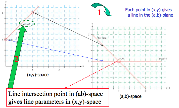
In the end, every parameter pair $(a, b)$ with a corresponding accumulator value exeding some threshold constitutes a line in $xy$ space.

Note that this only require $n_f n_a$ (where $n_a$ is the size of $\mathcal{A}$), while still a bit, it is much better than in the naive approach.

There are several problems with the cartesian way of describing lines, vertical lines would imply infinite parameter values, and in general, the range of the parameters are a problem. In stead we use polar coordinates, which is the perferred way.

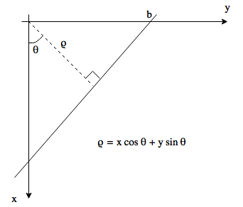
Straight line, polar coordinates

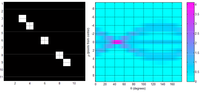
Every line in $xy$ space could be described in polar coordinates by $\rho = x\cos\theta + y\sin\theta$, where we have convenient boundaries for the parameters, $\rho \in [-d, d]$ and $\theta \in [0, \pi]$, where $d = \max_{i,j}\{ ||(x_i,y_i) - (x_j,y_j)||\}$. For the foreground class $F$, create a grid $\mathcal{G} = \mathcal{R} \times \Theta = \{\rho_1, ..., \rho_{n_\rho}\} \times \{\theta_1, ..., \theta_{n_\theta}\}$ which is called the accumulator grid, this is two-dimensional as there are two parameters ($\rho$ and $\theta$) needed to describe a line in $xy$ space. The values of the sets $\mathcal{R}$ and $\Theta$ are now bounded by the aforementioned ranges for the two parameters.

Figure 2: Polar representation of a line.

Traverse every element $(x_i, y_i)$ in $F$, and for each element, traverse every $\theta^* \in \Theta$ and compute $\rho' = x_i \cos\theta^* + y_i\sin\theta^*$. With some metric, find the the closest $\rho$ in $\mathcal{R}$, $\rho^* = \arg\min_{\rho \in \mathcal{R}}\{||\rho' - \rho||\}$.

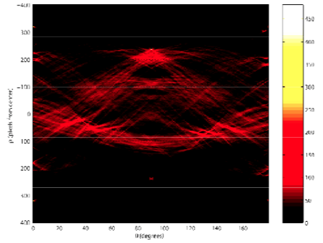
While, in the $xy$ case above we saw straight lines in the parameter space, we now see sinusoidals. As before, we have a accumulator function $A(\rho, \theta)$ for every $(\rho, \theta) \in \mathcal{G}$. Its initial value is zero for all parameter tuples. For every iteration explained above, $A(\rho^*, \theta^*)$ increments with one. Since we are sampling all points for a certain $(\rho, \theta)$ tuple, we will have many sinusoidals in the parameter space, and as with the straight lines discussed above, their intersection frequency in a cell is equivalent with the value of the accumulator function.

In the end, every parameter pair $(\rho, \theta)$ with a corresponding accumulator value exeding some threshold constitutes a line in $xy$ space.

Figure 3: Shapes in xy-space and corresponding parameter space accumulator (polar coordinates).

Figure 4: Example of parameter space accumulator values (polar coordinates).

Utilizing full gradient information

The images we are analysing, are already preprocessed with some edge detector, for example a low pass filter followed by a gradient filter. With the gradient filter it is common to get the vertical $g_x$ and the horizontal $g_y$ from the filtering, and then computing the gradient magnitude image $g_{mag} = \sqrt{g_x^2 + g_y^2}$ and the gradient direction image $g_{dir} = \tan^{-1}\left(\frac{g_y}{g_x}\right)$ (remember the rotated coordindate system that I am using for images). The idea is to, instead of, for each $\rho$ checking each angle $\theta$, we will instead accumulate only the direction $\theta = g_{dir}(x,y)$ for the particular edge index $(x,y)$. With this, we will not need to check as many parameters, and will get points in the parameter space in stead of sinusoudals.

Randomized Hough Transform

There are several problems with the ordinary Hough Transform, there are many redundant comparisons which effects the computation effort, and it would be great to somehow reduce the number of unnecessary searches. This is the main motivation behind the randomized Hough transform. I will describe it in brief below, and for a more extensive stydy, see this article from (Xu and Oja, 2009).

Pick a sufficient number of points in $F$ depending on the object that you are to detect (for lines you pick two, for circles you pick three etc.). Construct a line between the points, and find the parameter values for this line. Then accumulate the accumulator function for these parameter values. If there already exist an accumulator function for this parameter tuple (or a neighbouring tuple), increment it and set the new parameter tuple it is representing to some weighted average between the old and the new, then delete the old. If it does not exist, create it for this point, and set its value to 1. If the corresponding accumulator function has a sufficient value, put the parameter tuple into a set of candidate solutions. If the number of tuples in the set is above some threshold, examine all tuples in the set, and see if there are sufficient number of elements in the original image that can be expressed by this parameter tuple, if yes, store it as a solution, and delete its image elements from the image. If not, discard this solution. Return to start and pick a new set of image elements.

Pseudocode

• $s(x;\phi) = 0$ is a representation of an object in $x$-space.
• $t(\phi;x) = 0$ is a representation of the corresponding object in $\phi$-space.
• $F$ is a set of foreground pixels in $x$-space.
• $S$ is a set of solution parameters $\phi$, initially empty.
• $K$ is a set of non-solution parameters $\phi$, initially empty.
• $T_1$ and $T_2$ are predefined positive thresholds.
• $A(\phi)$ is the accumulator value for parameter $\phi$.
• while True
  • Pick a sufficient (2 for line, 3 for circle etc) number of points $\{x \in F\}$.
  • Compute parameters $\phi$ using $t(\phi; x) = 0$.
  • if $\phi \in K \cup S$
    • Contiunue from start and pick a new point.
  • else
    • if $A(\phi) > 0$
      • Increment count for this parameter: $A(\phi) \gets A(\phi) + 1$
      • Set candidate solution parameter: $\phi_{cand} = \phi$
    • else if $A(\phi') > 0$ for some $\phi' \in Neigh(\phi)$
      • Compute an average parameter $\phi'' = \frac{1}{2}(\phi + \phi')$
      • Insert it to the accumulator, and increment the count: $A(\phi'') = A(\phi') + 1$
      • Delete $A(\phi')$
      • Set candidate solution parameter: $\phi_{cand} = \phi''$
    • else
      • Insert this value to the accumulator with count 1: $A(\phi) = 1$
      • Set candidate solution parameter: $\phi_{cand} = \phi$
    • end if
    • if $A(\phi_{cand}) > T_1$
      • if $size(F \cap \{x' : t(\phi_{cand};x') = 0 \}) > T_2$
        • We found a solution: $S \gets S \cup \phi_{cand}$
        • Delete it from $F$: $F \gets F \setminus \{x' : t(\phi_{cand};x') = 0\}$
      • else
        • Blacklist it: $K \gets K \cup \phi_{cand}$
      • end if
    • end if
  • end if
  • if (max num iterations is reached) or ($F = \emptyset$)
• end while