Shape representation

Chain code

Chain code is a method of describing the shape of the boundary of an object in an image, we use the term chain code although its proper name is Freeman chain code. The idea is to traverse the boundary of the object, and for every new pixel, transcript the direction we traveled to reach this object.

It is common to denote the code relative to either a 4-connected neighbourhood or a 8-connected neighbourhood, and we have two major classes: absolute chain code and relative chain code. In both cases, the code consists of directions (referring to the enumerated directions in Figure 1) that you need to follow in order to traverse the boundary.

Figure 1: 4-connected and 8-connected neighbourhoods.

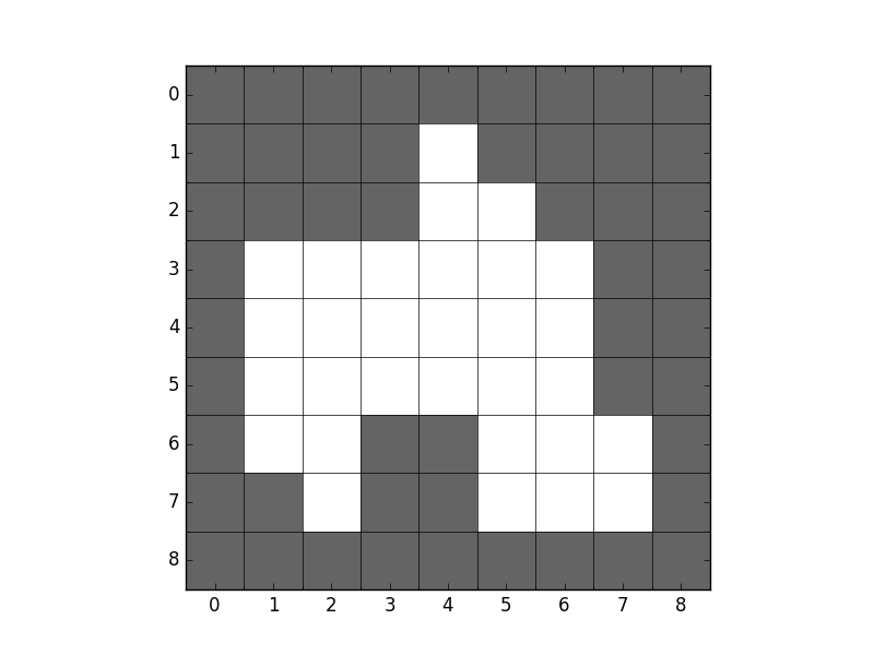
I will explain the different terms through examples, and the example figure we will use is a simple binary $9 \times 9$ image, where white is the color of the object which boundary we shall describe.

Figure 2: Example image with a white object.

Absolute chain code

In an absolute chain code, we always denote the direction relative to the orientation of the object we are investigating, using the directions in Figure 1 as they are. This is in contrast to a relative chain code, where a direction [^1] is fixed as forward, and when we traverse the object boundary, we always denote the new direction relative to our current forward facing direction.

Regular chain code

When transcribing chain code, we must select a starting point, say the leftmost pixel in the first row of the object (i.e. the pixel at [1, 4] in our example). Then, we traverse the boundary in a clockwise direction, from pixel to pixel, according to the connectivity we have selected. See implementation details for a more thorough walkthrough.

For a 4-connected neighbourhood, the next pixel is straight down at [2, 4], therefore the first number in our chain code would be 3. The next pixel is to the right [2, 5], making the next number in the chain code 0. Continuing this all the way around to our starting position gives the following chain code

$c^4 = (3,0,3,0,3,3,3,0,3,2,2,1,1,2,2,2,3,3,1,2,1,1,1,0,0,0,1,1).$

In a 8-connected neighbourhood, the first pixel after the starting position is at [2, 5], so our first number in the chain code is a 7. The next boundary point is [3, 6], making the next number in the chain code another 7. In the end we end up with

$c^8 = (7,7,6,6,7,6,4,4,2,3,4,5,6,3,2,2,2,0,0,1,2).$

Start position invariant chain code

In our example above, we chose a start position and developed our chain code from it. When describing the shape, we would rather have the code to be invariant to this starting point. The rule we follow is termed as forming the “integer of minimum magnitude” of our code, or performing a minimum circular shift. What is meant by this is that we think of the chain as beeing connected in the edges (forming a closed circle), and rotating the circle until you get a configuration that would form the smallest integer if you interpreted the numbers in the chain as digits in a integer. We denote this normalizing operator with $S: \mathbb{N}^N \to \mathbb{N}^N$ , where $N$ is the length of the chain code.

In our 4-connected chain, we see that there is a part at the end with the succession (…, 0, 0, 0, 1, …), and, since it starts with a lot of low numbers, are the part that, if put in the front would create the smallest integer

$S(c^4) = (0,0,0,1,1,3,0,3,0,3,3,3,0,3,2,2,1,1,2,2,2,3,3,1,2,1,1,1).$

Likewise, with the 8-connected chain we get

$S(c^8) = (0,0,1,2,7,7,6,6,7,6,4,4,2,3,4,5,6,3,2,2,2).$

The point is that, wherever you chose to start transcribing, you can do this circular transform and end up with the same code.

Rotation invariant chain code.

After all, we are describing the shape of an object, a property that should be invariant to the rotation of the object; the shape is the same even if it is rotated.

In order to make the chain code invariant to rotation, we create a code based on the difference between elements in the code we are normalizing, something which is called the first difference of the chain code. Let us denote this function with $R: \mathbb{N} \to \mathbb{N}$ for element wise operations, with a slight abuse of notation we also use $R$ when we operate on full chain codes. With this, each element in our new rotation invariant code, is computed as

$R(c^k_i) = \begin{cases} \text{mod}\{c^k_{i+1} - c^k_i, k\} ,& \quad \text{ for } 0 \le i < N-1 \\ \text{mod}\{c^k_0 - c^k_i, k\} ,& \quad \text{ for } i = N-1 \end{cases}$

where $k \in \{4, 8\}$ is the neihbourhood connectivity. Following this, we can make our chain codes from above rotation invariant (and start-point invariant)

$\begin{align} c^4 &= (3,0,3,0,3,3,3,0,3,2,2,1,1,2,2,2,3,3,1,2,1,1,1,0,0,0,1,1), \\ R(c^4) &= (1, 3, 1, 3, 0, 0, 1, 3, 3, 0, 3, 0, 1, 0, 0, 1, 0, 2, 1, 3, 0, 0, 3, 0, 0, 1, 0, 2), \\ S(R(c^4)) &= (0,0,1,0,2,1,3,0,0,3,0,0,1,0,2,1,3,1,3,0,0,1,3,3,0,3,0,1), \end{align}$

and for the 8-connected case

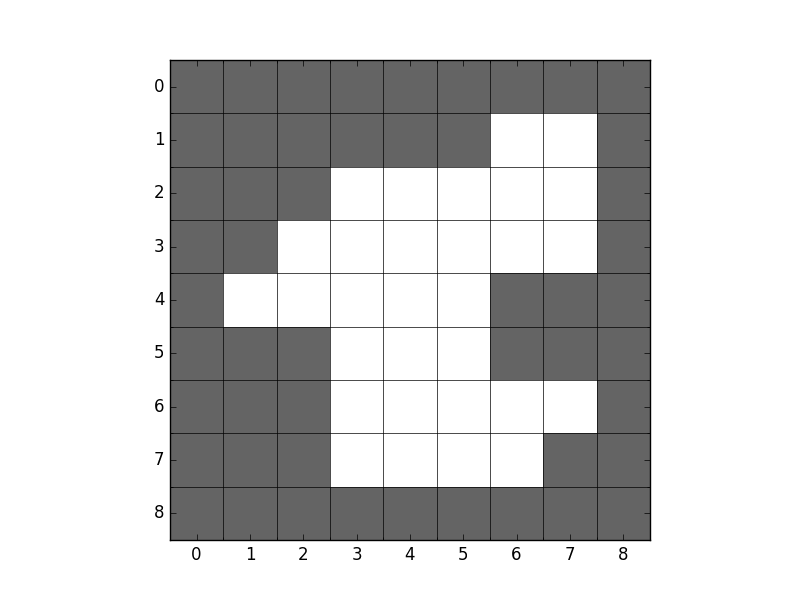
$\begin{align} c^8 &= (7,7,6,6,7,6,4,4,2,3,4,5,6,3,2,2,2,0,0,1,2), \\ R(c^8) &= (0, 7, 0, 1, 7, 6, 0, 6, 1, 1, 1, 1, 5, 7, 0, 0, 6, 0, 1, 1, 5), \\ S(R(c^8)) &= (0,0,6,0,1,1,5,0,7,0,1,7,6,0,6,1,1,1,1,5,7). \end{align}$

Figure 3: Object from Figure 2 rotated 90 degrees.

To see that this is really the case, let us compute the chain code from the rotated object in Figure 3, normalize it w.r.t. starting point, and then w.r.t. rotation. Starting at [1, 6] going clockwise, we get

$\begin{align} c^4 &= (0,3,3,2,2,3,3,3,0,0,2,3,2,2,2,1,1,1,2,2,0,1,0,1,0,0,0,1), \\ S(c^4) &= (0,0,0,1,0,3,3,2,2,3,3,3,0,0,2,3,2,2,2,1,1,1,2,2,0,1,0,1), \\ R(S(c^4)) &= (0,0,1,3,3,0,3,0,1,0,0,1,0,2,1,3,0,0,3,0,0,1,0,2,1,3,1,3), \\ S(R(S(c^4)) &= (0,0,1,0,2,1,3,0,0,3,0,0,1,0,2,1,3,1,3,0,0,1,3,3,0,3,0,1). \end{align}$ $\begin{align} c^8 &= (0,6,6,4,5,6,7,0,5,4,4,4,2,2,3,4,1,1,0,0,1), \\ S(c^8) &= (0,0,1,0,6,6,4,5,6,7,0,5,4,4,4,2,2,3,4,1,1), \\ R(S(c^8)) &= (0,1,7,6,0,6,1,1,1,1,5,7,0,0,6,0,1,1,5,0,7), \\ S(R(S(c^8))) &= (0,0,6,0,1,1,5,0,7,0,1,7,6,0,6,1,1,1,1,5,7). \end{align}$

which, after normalizing for starting point, is identical to the one we got from the object before it was rotated. Note that in the example above, we applied the rotation normalization on a chain code already normalized for starting point. We could just as well have applied it on an unnormalized chain code, since in order to see that they are identical, the rotation invariant code need also to be normalized for starting point. This stems from the fact that the operations for starting point invariance and rotation invariance are associative, meaning that it does not matter in which order we apply them.

Relative chain code

As mentioned above, in relative chain coding, we always denote the new direction relative to a forward direction. The resulting code is naturally dependent on this choice of forward, and in the lecture slides, the upward (or north) direction is used (that is, 1 for a 4-connected system and 2 for a 8-connected system). I will, however use 0 as the forward direction in this notes, and in the solution proposal, to keep it the same for both systems (and also, I personally think 0 is a more natural choice). In my opinion one can use whatever seems natural as long as one is consistent and state the choice explicitly. The difference in the resulting chain code after applying different definitions of the forward direction is just a circular shift equal to the difference between the chain codes modulo the number of neighbours in the neigbourhood system.

Starting at position [1, 4], we get the following using 0 as forward:

$c^4 = (0,1,3,1,3,0,0,1,3,3,0,3,0,1,0,0,1,0,2,1,3,0,0,3,0,0,1,0)$

Notice that if we where to continue after the last pixel, we would not put a 0 (the start of the chain), but rather a 2 (in the 4-connected case). Therefore it is common to change the first number in the chain code to whatever the next number would have been if we were to continue the chain, giving

$c^4 = (2,1,3,1,3,0,0,1,3,3,0,3,0,1,0,0,1,0,2,1,3,0,0,3,0,0,1,0)$

in our case. Normalizing w.r.t. starting position follows the same rule as for the absolute chain code, yielding

$S(c^4) = (0,0,1,0,2,1,3,0,0,3,0,0,1,0,2,1,3,1,3,0,0,1,3,3,0,3,0,1).$

This seems very familiar, and is in fact the same rotation invariant code we found with absolute chain coding after normalizing for starting point. To check that it is relly rotation invariant, we can double check with our rotated object from Figure 3

$\begin{align} c^4 = (3,3,0,3,0,1,0,0,1,0,2,1,3,0,0,3,0,0,1,0,2,1,3,1,3,0,0,1), \\ S(c^4) = (0,0,1,0,2,1,3,0,0,3,0,0,1,0,2,1,3,1,3,0,0,1,3,3,0,3,0,1). \end{align}$

This is also the case for the 8-connected neighbourhood, which I leave to the reader to check.

Implementation of absolute chain code

Here, I will explain in detail how to compute a chain code from a binary image containing an object. This will implement the regular chain code (with reference to the naming above), and normalization w.r.t. starting position and rotation can be easily computed from the regular one (following the corresponding explanations above). For a full example code in python, you can download the script chain_code.py here.

Start pixel

When traversing the object in a clockwise direction, and also search the local neighbourhood in a clockwise direction, we must start at the top left pixel in the object. That is, the first column in the first row containing an object pixel.

Local neighbourhood search

Around each current boundary point, we search the local neighbourhood (corresponding to the chosen connectivity) in a clockwise direction. When implementing this, we must know where in the local neighbourhood to start the search. If $c_{n-1}$ is the direction we used to arrive at our current pixel, then the start position $s$ (relative to a neighbourhood configuration), can be computed as

$s = \text{mod}(c_{n-1} - 3, 4)$

for a 4-connected neighbourhood, and

$s = \begin{cases} \text{mod}(c_{n-1} - 6, 8), & \text{ if } c_{n-1} \text{ is odd} \\ \text{mod}(c_{n-1} - 7, 8), & \text{ if } c_{n-1} \text{ is even} \end{cases}$

for a 8-connected neighbourhood. If we are at the beginning, and do not have any previous directions yet, we initialize this with 0 if we are using a 4-connected neighbourhood, and to 7 if we are using a 8-connected neighbourhood.

Skeletons

Gonzales and Woods (section 11.1.7) defines the skeleton or the medial axis of an object as.

For each point $p$ in a region $R$ , we find its closest neighbor at the boundary $B$ . If $p$ has more than one such neighbor, it is said to belong to the medial axis (skeleton) of $R$ .

Binary region thinning algorithm

Direct implementation of the definition above is computationally expensive, so G&W propose a way to thin binary regions.

Object points are assumed to have the value 1 while background points have the value 0. A boarder point is any pixel with a value 1 having at least one background pixel as a neighbour.

The algorithm consists of traversing the boundary of the object, deleting suitable points (setting them to 0), update the object, and do the procedure again.

Pseudocode

Assume a region $R$ with border $B$ consisting of pixels $p$ .
while not converged
- Apply Step 1 to every $p \in B$ , flagging points for deletion.
- Delete the flagged points from $R$ , thus updating $R$ (and $B$ ).
- Apply Step 2 to every $p \in B$ , flagging points for deletion.
- Delete the flagged points from $R$ , thus updating $R$ (and $B$ ).
- If no points has been deleted, terminate the algorithm.

With the 8-connected neighbourhood defined as

$\begin{array}{|c|c|c|} \hline p_9 & p_2 & p_3 \\ \hline p_8 & p_1 & p_4 \\ \hline p_7 & p_6 & p_5 \\ \hline \end{array}$

around a border point at $p_1$ , we define Step 1 and Step 2 as follows.

Step 1

This step flags a contour point $p_1$ for deletion if the following conditions are satisfied

a) $2 \le N(p_1) \le 6$

b) $T(p_1) = 1$

c) $p_2 \cdot p_4 \cdot p_6 = 0$

d) $p_4 \cdot p_6 \cdot p_8 = 0$

Here, $N(p_1)$ denote the number of nonzero neighbours of $p_1$

$N(p_1) = \sum_{i=2}^9 p_i$

where $p_i \in \{0, 1\}$ is the value at this position. $T(p_1)$ is the number of $0-1$ transitions in the ordered sequence $p_2, p_3, ..., p_8, p_9, p_2$ . As an example, for the neighbourhood

$\begin{array}{|c|c|c|} \hline 0 & 0 & 1 \\ \hline 1 & p_1 & 0 \\ \hline 1 & 0 & 1 \\ \hline \end{array}$

$N(p_1) = 4$ and $T(p_1) = 3$ .

Step 2

The same as Step 1, except point c) and d) is changed. That is, this step flags a contour point $p_1$ for deletion if the following conditions are satisfied

a) $2 \le N(p_1) \le 6$

b) $T(p_1) = 1$

c) $p_2 \cdot p_4 \cdot p_8 = 0$

d) $p_2 \cdot p_6 \cdot p_8 = 0$