Object feature extraction - shape descriptors

Image moments

Borrowing nomenclature from probability theory, we can define certain moments based on the intensity value of the image. Moments are useful for computing properties such as centroid and area of an object. We will list the general case, where $f$ is a discrete image taking grayscale values.

Raw moments

The raw moments of $f$ of order $(p + q)$ are defined as

$m_{pq} = \sum_x \sum_y x^p y^p f[x, y].$

From this, we can e.g. compute the centroid $(c_x, c_y)$

$\begin{align} c_x &= \frac{m_{10}}{m_{00}} \\[0.5ex] c_y &= \frac{m_{01}}{m_{00}}, \end{align}$

where, in case of a binary image, $m_{00}$ is the area of the foreground object.

Central moments

Central moments are moments that are centered around the centroid, and thus invariant to translation

$\mu_{pq} = \sum_x \sum_y (x - c_x)^p (y - c_y)^p f[x, y]$

With this, we can compute the covariance matrix

$Cov(f) = \frac{1}{\mu_{00}} \left( \begin{array}{cc} \mu_{20} & \mu_{11} \\ \mu_{11} & \mu_{02} \end{array} \right)$

from which we can compute eigenvectors. Now, the angle of eigenvector corresponding to the largest eigenvalue is the angle of the major axis of the object, which we can define as the orientation of the object.

We will here derive some of the lower central moments.

Obviously,

$\mu_{00} = m_{00}.$

For the first order central moments,

$\begin{align} \mu_{10} &= \sum_x \sum_y (x - c_x) f[x, y] \\[0.5ex] &= m_{10} - c_x m_{00} \\[0.5ex] &= 0, \end{align}$

and likewise, $\mu_{01} = 0$ .

$\begin{align} \mu_{11} &= \sum_x \sum_y (x - c_x)(y - c_y) f[x, y] \\[0.5ex] &= m_{11} - c_y m_{10} - c_x m_{01} + c_x c_y m_{00} \\[0.5ex] &= m_{11} - \frac{m_{10}m_{01}}{m_{00}} \\[0.5ex] &= m_{11} - c_x m_{01} \\[0.5ex] &= m_{11} - c_y m_{10}. \end{align}$

And, finaly for the second order moments

$\begin{align} \mu_{20} &= \sum_x \sum_y (x - c_x)^2 f[x, y] \\[0.5ex] &= m_{20} - 2 c_x m_{10} + c_x^2 m_{00} \\[0.5ex] &= m_{20} - c_x m_{10}, \end{align}$

and in a similar manner, $\mu_{02} = m_{02} - c_y m_{01}$ .

Normalized central moments

We can in addition to translation invariance obtain scale invariance with normalized central moments

$\eta_{pq} = \frac{\mu_{pq}}{\mu_{00}^{1 + \frac{p+q}{2}}}, \quad p+q \ge 2$

Hu moments

Hu moments are invariant to translation, scale, and rotation, and are stated below for completion.

$\begin{align} \zeta_1 &= \eta_{20} + \eta_{02} \\[0.5ex] \zeta_2 &= (\eta_{20} - \eta_{02})^2 + 4\eta_{11}^2 \\[0.5ex] \zeta_3 &= (\eta_{30} - 3\eta_{12})^2 + (3\eta_{21} - \eta_{03})^2 \\[0.5ex] \zeta_4 &= (\eta_{30} + \eta_{12})^2 + (\eta_{21} + \eta_{03})^2 \\[0.5ex] \zeta_5 &= (\eta_{30}-3\eta_{12})(\eta_{30}+\eta_{12})\left[(\eta_{30}+\eta_{12})^2-3(\eta_{21}+\eta_{03})^2\right] + (3\eta_{21}-\eta_{03})(\eta_{21}+\eta_{03})\left[3(\eta_{30}+\eta_{12})^2-(\eta_{21}+\eta_{03})^2\right] \\[0.5ex] \zeta_6 &= (\eta_{20}-\eta_{02})\left[(\eta_{30}+\eta_{12})^2-3(\eta_{21}+\eta_{03})^2\right] + 4\eta_{11}(\eta_{30}+\eta_{12})(\eta_{21}+\eta_{03}) \\[0.5ex] \zeta_7 &= (3\eta_{21}-\eta_{03})(\eta_{30}+\eta_{12})\left[(\eta_{30}+\eta_{12})^2-3(\eta_{21}+\eta_{03})^2\right] - (\eta_{30}-\eta_{12})(\eta_{21}+\eta_{03})\left[3(\eta_{30}+\eta_{12})^2-(\eta_{21}+\eta_{03})^2\right] \\[0.5ex] \end{align}$

Example

In this example, we will find the centroid and the direction of a swarm of birds, or at least of the birds in the image bird_swarm.jpg, which can be found here.

Figure 1: Swarm of birds.

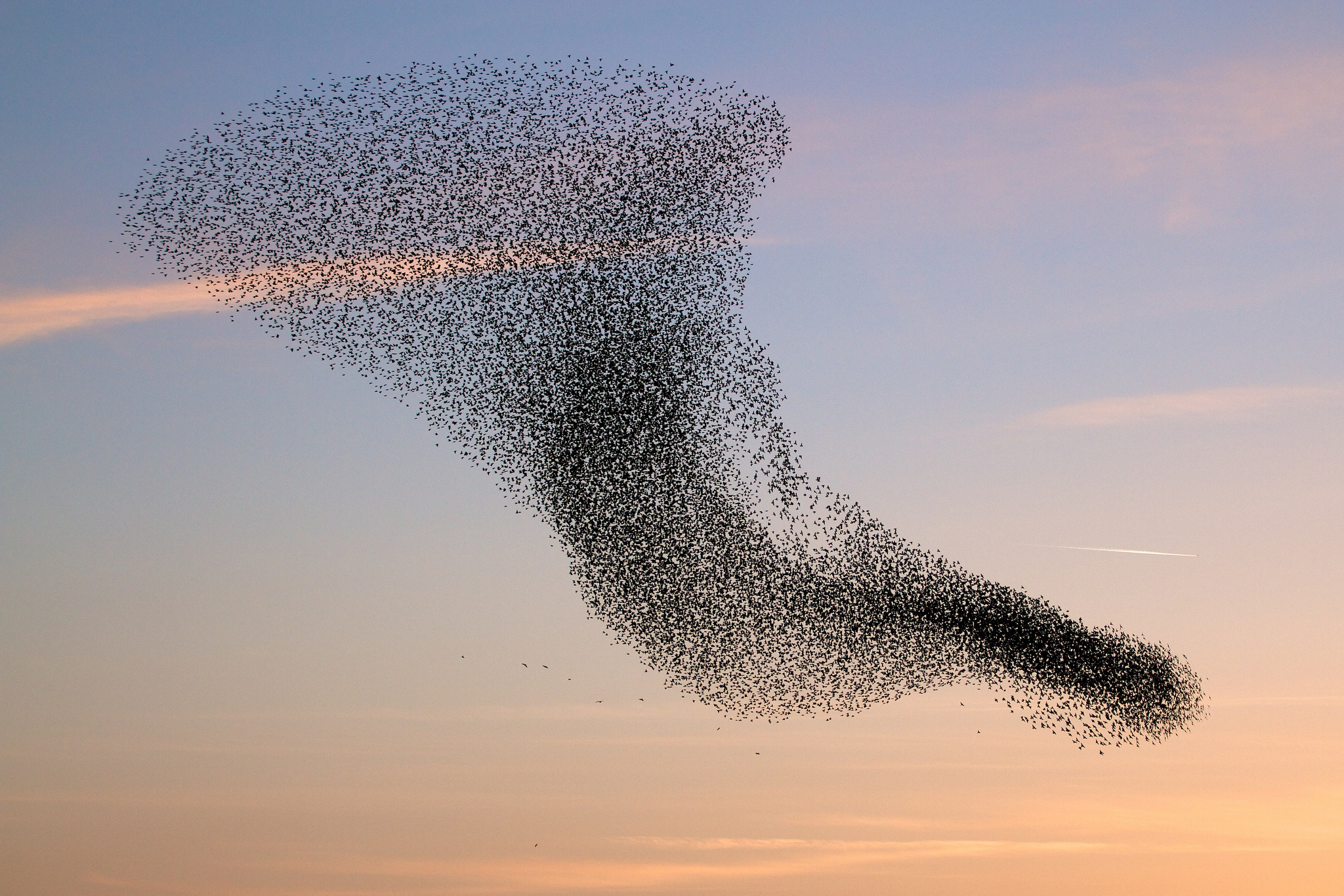
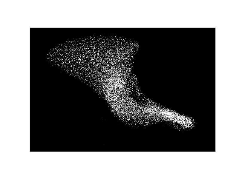
We first read in the image, and threshold it to get the birds as foreground.

import numpy as np
import matplotlib.pyplot as plt
import cv2

image_file = '../../bird_swarm.jpg' # Change this to your location
img = cv2.imread(image_file, cv2.IMREAD_COLOR)

gl_img = cv2.cvtColor(img, cv2.COLOR_BGR2GRAY)
thresh_img = gl_img < 50
plt.imshow(thresh_img, cmap='gray')
plt.xticks([]), plt.yticks([])
plt.show()

Figure 2: Thresholded swarm, birds as foreground.

Then, we compute the moments, and note that $f[x, y] = 0$ for background and $f[x, y] = 1$ for foreground. Notice also that we use ( $x$ , $y$ ) as in a regular cartesian coordinate convention.

m00 = m01 = m10 = m11 = m20 = m02 = m21 = m12 = 0
height, width = thresh_img.shape
for y in range(height):
  for x in range(width):
    m00 += thresh_img[y, x]
    m10 += x*thresh_img[y, x]
    m01 += y*thresh_img[y, x]
    m11 += x*y*thresh_img[y, x]
    m20 += x*x*thresh_img[y, x]
    m02 += y*y*thresh_img[y, x]
    m21 += x*x*y*thresh_img[y, x]
    m12 += x*y*y*thresh_img[y, x]

Next, we compute the centroid

cx = m10 / m00
cy = m01 / m00
print('Centriod: ({0:.2f}, {1:.2f})'.format(cx, cy))

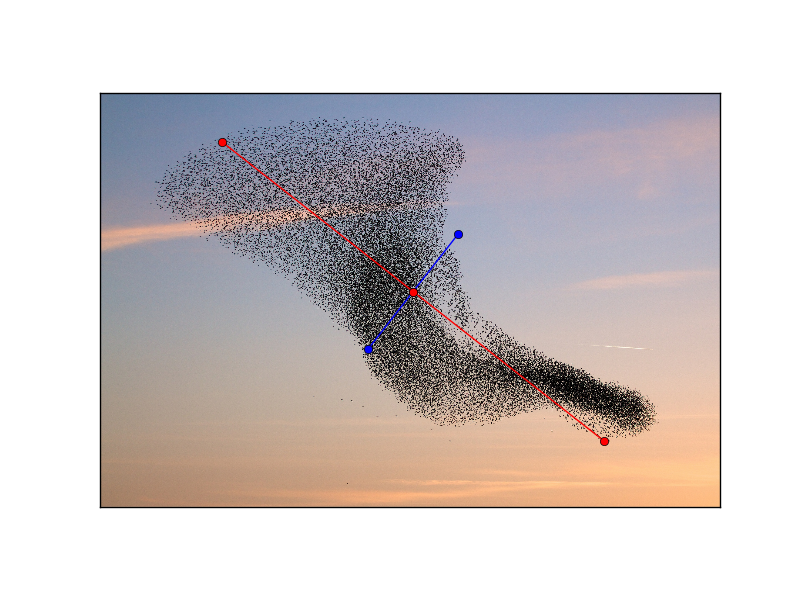
which outputs Centriod: (1034.36, 654.48). Using the central moments above, we can also compute the angle of the major axis of the swarm, relative to the horizontal coordinate axis. Note that we use np.arctan2(...) to make our life easier, quadrant-wise.

mu00 = m00
mu11 = m11 - cx*m01
mu20 = m20 - cx*m10
mu02 = m02 - cy*m01
theta = 1/2*np.arctan2(2*mu11/mu00, (mu20 - mu02)/mu00)
print('Angle {0:.2f}'.format(theta*180/np.pi))

which prints Angle: 38.05. We now plot the major and minor axis (with arbitrary length) on top of the original image to illustrate the location of the centriod and the angle.

rho = 800
dx_major = rho*np.cos(theta)
dy_major = rho*np.sin(theta)
dx_minor = 0.3*rho*np.cos(theta - np.pi/2)
dy_minor = 0.3*rho*np.sin(theta - np.pi/2)

plt.imshow(cv2.cvtColor(img, cv2.COLOR_BGR2RGB))
plt.plot([cx-dx_minor, cx, cx+dx_minor], [cy-dy_minor, cy, cy+dy_minor], 'bo-')
plt.plot([cx-dx_major, cx, cx+dx_major], [cy-dy_major, cy, cy+dy_major], 'ro-')
plt.xticks([]), plt.yticks([])

# Remove redundant space left by the plt.plot() commands
axes = plt.gca()
axes.set_xlim([0, width])
axes.set_ylim([height, 0])

plt.show()

Figure 3: Bird swarm with centroid, major axis (red) and minor axis (blue).

Region properties

Based on the contour of an object, we will here show how to estimate the area and perimeter of this object. For reference, see e.g. (Yang, Albregtsen, Lønnestad, Grøttum (1994)) Methods to estimate areas and perimeters of blob-like objects: a comparison.

Properties from chain code

For 8-connected chain code, we can approximate the area an perimeter using the following formulas.

Here, $N$ is the length of the chain code, $(\Delta x)_i$ and $(\Delta y)_i$ indicates the change in direction of $x$ and $y$ , respectively, from chain code element $c_i$ . E.g. for $c_i = 6$ , $(\Delta x)_i = -1$ and $(\Delta y)_i = 0$ . $n_e$ and $n_o$ is the number of even and odd chain code elements, and $n_c$ is the number of corners in the chain code. $y_i$ is the $y$ position at element $i$ (this can be initialized to an arbitrary value as the chain code should be translation invariant).

Freeman

$\begin{align} P_F &= n_e + n_o\sqrt{2}\\[0.5ex] A_F &= \sum_{i = 0}^{N-1} (\Delta x)_i \left[\text{mod}\{y_{i-1}, N\} + \frac{1}{2}(\Delta y)_i \right] \end{align}$

Vossepoel and Smeulders

$P_{VS} = 0.980 n_e + 1.406 n_o - 0.091 n_c$

Kulpa

$P_{K} = \frac{\pi}{8} \left(1 + \sqrt{2}\right) \left(n_e + n_o \sqrt{2} \right)$

Properties from bit quads pattern matching

We can also estimate the area and perimeter of an object by matching local windows in an image with some patterns that we will define below. For a given list of patterns $P$ and a local window $W$ in an image, we match the window to any of the patterns in the pattern list. We do this for all local windows in an image, and accumulate the number of matches in a count variable $n(P)$ . Explicitly, if our pattern is $2\times 2$ , we select a $2\times 2$ window, beginning with pixels $[0,0], [0,1], [1,0], [1,1]$ , the next windown will be one pixel to the right, and we continue in this sliding fashion until the whole image is covered. Note that it is important that the region you are examining is filled.

Patterns

The following (list of) patterns is defined:

Single

$S = [1].$

Horizontal

$H = \left[ \begin{array}{cc} 0 & 1 \end{array} \right].$

Vertical

$V = \left[ \begin{array}{c} 0 \\ 1 \end{array} \right].$

Qadratic 0

$Q_0 = \left[ \begin{array}{cc} 0 & 0 \\ 0 & 0 \end{array} \right].$

Qadratic 1

$Q_1 = \left[ \begin{array}{cc} 1 & 0 \\ 0 & 0 \end{array} \right], \left[ \begin{array}{cc} 0 & 1 \\ 0 & 0 \end{array} \right], \left[ \begin{array}{cc} 0 & 0 \\ 0 & 1 \end{array} \right], \left[ \begin{array}{cc} 0 & 0 \\ 1 & 0 \end{array} \right].$

Qadratic 2

$Q_2 = \left[ \begin{array}{cc} 1 & 1 \\ 0 & 0 \end{array} \right], \left[ \begin{array}{cc} 0 & 1 \\ 0 & 1 \end{array} \right], \left[ \begin{array}{cc} 0 & 0 \\ 1 & 1 \end{array} \right], \left[ \begin{array}{cc} 1 & 0 \\ 1 & 0 \end{array} \right].$

Qadratic 3

$Q_3 = \left[ \begin{array}{cc} 1 & 1 \\ 0 & 1 \end{array} \right], \left[ \begin{array}{cc} 0 & 1 \\ 1 & 1 \end{array} \right], \left[ \begin{array}{cc} 1 & 0 \\ 1 & 1 \end{array} \right], \left[ \begin{array}{cc} 1 & 1 \\ 1 & 0 \end{array} \right].$

Qadratic 4

$Q_4 = \left[ \begin{array}{cc} 1 & 1 \\ 1 & 1 \end{array} \right].$

Qadratic diagonal

$Q_d = \left[ \begin{array}{cc} 1 & 0 \\ 0 & 1 \end{array} \right], \left[ \begin{array}{cc} 0 & 1 \\ 1 & 0 \end{array} \right].$

Property estimates

Referring to the patterns above, we can estimate the area and perimeter in a number of ways.

4-connected objects

$\begin{align} A_4 &= n(S) \\[0.5ex] P_4 &= 2n(H) + 2n(V). \end{align}$

Gray

$\begin{align} A_G &= \frac{1}{4}\left[n(Q_1) + 2n(Q_2) + 3n(Q_3) + 4n(Q_4) + 2n(Q_d)\right] \\[0.5ex] P_G &= n(Q_1) + 2n(Q_2) + n(Q_3) + 2n(Q_d) \end{align}$

Duda

$\begin{align} A_D &= \frac{1}{4}\left[n(Q_1) + 2n(Q_2) + \frac{7}{2}n(Q_3) + 4n(Q_4) + 3n(Q_d)\right] \\[0.5ex] P_D &= n(Q_2) + \frac{1}{\sqrt{2}}\left[n(Q_1) + n(Q_3) + 2n(Q_d) \right] \end{align}$