Classification of images can mean a lot of things, usually it is used in the context of classifying images based on the things in the image, e.g. “this is an image of a dog”, or “this is an image of a cat”.

This note is related to the exercise for this week, where the task is to partition an image according to different classes, also called image segmentation. More formally, the task is to assign a class $c \in \mathcal{C}$ to every pixel $s$ in an image $\mathcal{S}$, where $\mathcal{C}$ is set of classes in which it can belong.

In this note we will cover a univariate Gaussian classifier, utilizing one feature at a time, while multivariate classifiers will be covered later.

Univariate Gaussian classifier

Since this is a univariate classifier, every pixel $s$ will be associated with one observable or computable feature, $x$. We will use this feature $x$ to determine in which class $s$ belongs, or equivivalently, in which class the feature $x$ will belong. Let $\mathcal{X}$ denote the set of features associated with the image $\mathcal{S}$ such that each $s \in \mathcal{S}$ will have a unique feature $x \in \mathcal{X}$. Note that even though each pixel has an assosiated feature, the value of the feature can be shared by multiple pixels.

Probability model

For each pixel $s$ we will model its associated feature as a continuous random variable $X$ which range is in $\mathbb{R}$. Likewise, we will model the class as a discrete random variable $C$ which range is in $\mathcal{C}$. For $C$ we will have an a priori probability density (or simply prior) $p_C(c) = Pr(C = c)$ which is the probability of labeling $s$ with $c$ before any features are observed. Likewise, we have the probability density of $X$, $f_X(x) = Pr(X = x)$, and by total probability, this can be written as

Here, $f_{X,C}(x,c)$ is the joint probability of $X$ taking the value $x$ and $C$ taking the value $c$.

We now define the likelihood $f_{X|C=c}(x) = Pr(X = x | C = c)$ which is the probability of $X$ taking the value of $x$ if it indeed belongs to class $c$. With this, we can now define the a posteriori (or posterior) probability density

Note that the denominator is not dependent on the particular class $c$, and we can view this as simply a normalization factor. This is very convenient, as the true density of $X$ can be quite cumbersome to find (or at least express analytically and concise).

This posterior distribution is what we are after. It describes the probability of $C$ taking the value $c$ given that we have observed $X = x$. In our case; the probability that pixel $s$, with a corresponding feature $x$, belongs to class $c$.

Discrimination function

In this classification, we will label the pixel with the class which produces the largest posterior probability given the observations $x$. Formally, we define a discrimination function $a: \mathbb{R} \to \mathcal{C}$ to be the mapping from an observed feature $x$ to a class $c$,

where some equivalent and convenient representation was also included.

Gaussian distribution model

Up until now, we have not said anything about which distributions the random variables belong to, so we will specify them here. We assume that $C$ is uniformly distributed over $\mathcal{C}$,

where $n$ is the number of classes in $\mathcal{C}$. The conditional likelihood will be a univariate Gaussian $(X | C = c) \sim \mathcal{N} (x; \mu_c, \sigma_c)$

where $\mu_c$ is the feature mean of class $c$ and $\sigma_c$ is the feature variance of class $c$. Important: $\mu_c$ and $\sigma_c$ are the variables that are to be determined when training the classifier.

Note that the determination function $a$ is not dependent on the marginal density of $X$, so, as mentioned above, we will not specify it further. Since we have now described our distributions, we can revisit the discrimination function

where the last representation is what is actually implemented.

Training

In order to determine $\mu_c$ and $\sigma_c$, we need to have a training set $\mathcal{X}^t_c \subset \mathcal{X}$ for each class label $c$

This can e.g. be obtained by masking out the pixels of a feature image $\mathcal{S_x}$ belonging to the class $c$, for every class in $\mathcal{C}$.

We then estimate the class mean as

and the class variance estimate as

where $|\{\}|$ denotes the number of elements in the set. We use hat notation to emphasize that we are computing estimates of the actual class mean and variance.

Dataset partition

When a true classification is available, we can evaluate our proposed classifier against this reference classification, this is called supervised evaluation. On the same note, our classifier is a supervised classifier, since we are training it using a training set of labeled pixels to estimate the parameters in the classifier.

The dataset of labeled pixels is normally partitioned into a training set, a validation set, and a test set. The training set is used to train our classifier. The validation set is used to finetune or adjust hyperparameters, parameters that are a part of the classifier, but not trainable variables. The test set is used to evaluate the classifier.

Normally, the training set is the largest partition. The reason is simply that our classifier usually performs better when trained on a larger training set (up to some reasonable quantity). A classifier should be able to “learn what it is thaught”, meaning that it should perform good on cases it is trained on. But parhaps more importantly, it should generalize well, after all, we want to train a classifier so that we can use it on new examples. Training on a small training set often leaves our classifier overtrained, meaning that it perform well on data from the training set, but poorly on new data. And this is the point of a large training set, with it, we hope that the classifier sees enough examples from a large spectrum, such that it performs well on new data. Note that the data in the training set needs to span a wide variety, a large training set size is of no use if all examples in the training set are identical.

Classification

The procedure for classifying an image $\mathcal{S}$ is then to classify each pixel $s \in \mathcal{S}$ by evaluating the function $a(x)$ for the feature $x$ assosiated with the pixel $s$, and using the mean and covariance estimators obtained from the training.

More verbose, for each $s \in \mathcal{S}$, find the associated feature $x$ (e.g. obtained from a feature image $\mathcal{S}_x$). Then compute

for all classes $c \in \mathcal{C}$, and label $s$ with the class

Evaluation

After you have trained your classifier, that is, computed estimates $\hat{\mu_c}$ and $\hat{\sigma_c}$, you have your proposed classifier which you can use to classify (in our case) pixels in an image. One can imagine that we are trying out different classifiers, parhaps based on different features or training data, and in this case it is important to have a tool to quantify the success of the different classifiers.

As mentioned above, we evaluate our classifier on the test set partition of our labeled data. It is very important that the training set and test set are independent such that we actually test how the classifier work on new data, as a overtrained classifier would achieve good results on a test set resembling the training set, which is of little practical utility.

In this case it is common to compute a so called confusion matrix $M$ such that element $m_{c_r c_p}$ is the number of pixels labeled $c_r$ by the reference and labeled $c_p$ by our proposed classifier. Correctly classified pixels will be accumulated on the diagonal, and wrongly labeled off the diagonal.

Basic quantities

From this confusion matrix, we can compute a number of different evaluation metrics, but first, we must define some basic quantities. Let $N$ be the total number of pixels in our test set. Let $RP_c$ and $PP_c$ denote the total number of pixels in the test set labeled with class $c$ by the reference classifier, and the proposed classifier, respectively. Conversly, let $RN_c$ and $PN_c$ be the number of pixels not labeled $c$ by the reference and the proposal, respectively.

True positive

For class $c$, we let $TP_c$ denote the number of true positive pixels, that is, pixels that is labeled $c$ by both the reference and proposal classifier.

False positive

The number of false positive pixels for class $c$ is denoted $FP_c$, and it is the number of pixels labeled $c$ by the proposal, but not by the reference (here, we do not discriminate between different missclassifications).

where the sum is over all classes $k \in \mathcal{C}$ except for the class $c$.

False negative

The number of false negative pixels for class $c$ is denoted $FN_c$, and is the number of pixels labeled $c$ by the reference but not by the proposal classifier.

True negative

The number of true negative pixels for class $c$ is denoted $TN_c$. and is the number of pixels not labeled $c$ by both the reference and the proposal classifier.

Convenience relations

From the basic quantites above, we can list some sanity checks:

Probabilistic interpretation

If we normalize the confusion matrix, it can be interpreted like an estimate for the joint probability mass function between the reference and proposed classification. Let $Y_R$ and $Y_P$ be discrete random variables taking values in $\mathcal{C}$, and let them model the label given by the reference, and proposal, respectively. And with some abuse of notation, let $P$ denote some probability measure, then the following interpretation can be made of the relative quantities defined in the table.

Compound evaluation metrics

Here, we will list some common evaluation metrics used to evaluate classification performance. What metric (or ensamble of different metrics) to use really depend on the application of your classifier, but some general words can be said of each of them.

True positive rate (sensitivity)

Expression:

Probabilistic interpretation:

This measures the fraction of the reference positive you where able to correctly classify. This does not take into account wrong classifications, and a classifier classifying everything to class $c$ would achieve perfect sensitivity.

True negative rate (specificity)

Expression:

Probabilistic interpretation:

This measures how well you hit the target, caring only of the missclassified region. A consequence of this is that if your classifier did not classify anything with the label $c$, this classifier would achieve perfect specificity. Also, it is not invariant to prevalence, meaning that increasing the sample size would improve the result.

Positive predictive value (precision)

Expression:

Probabilistic interpretation:

This measures the what proportion of the region the proposed classifier labeles with a class label actually belongs to the class. Or what is the probability of a positive labeled outcome actually is positive. This metric is not independent of prevalence, and increasing the number of reference positive would likely increase the precision (all else equal).

Negative predictive value

Expression:

Probabilistic interpretation:

Conversly, this measures the probability of a proposed negative result actually being negative. But as the above metrics, this one is not independent of prevalence, and you could get a better performance by increasing the sample size.

Rand accuracy

Expression:

Probabilistic interpretation:

A often used metric that takes into account both true positives and true negatives. This is also not independent of prevalence, and adds little information in terms of evaluating a classifier. Classifying rare instances would automatically achieve high accuracy, a property which is somewhat undesirable for a classifier evaluator.

Jaccard index (intersection over union)

Expression:

Probabilistic interpretation:

A classifier often used in evaluation of segmentation methods. This is invariant to sample size, but does not take into account the correctly negative labeled outcomes. Depending on the application, this is not as hopeless as the metrics discussed above.

Dice similarity coefficient

Expression:

Probabilistic interpretation:

Essentially the same as the Jaccard index, but measures the fraction “number of true positive” over the “mean number classified by the reference and proposal” in stead of over the “number classified by the reference and proposal in union”.

Area under ROC

Expression:

Probabilistic interpretation:

This measures the area under the receiver operating characteristic curve, and as can be seen from the expression, is an average between the sensitivity and the specificity. Hence, it inherits the properties of those metrics, which was discussed above. Contrary to the metrics above, a value of 0.5 represent the result of a classifier classifying at random, and thus completely useless.

Development plot

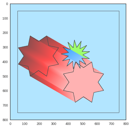
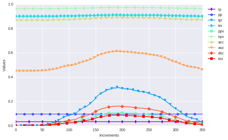
Here is a toy example to illustrate how the different metrics discussed above changes when a proposal star object is “passing through” a reference star object (from dark to bright colors).

Figure 1: Black square: region of interest. Red region: only classified by the proposal segmentation. Green region: only classified by the reference segmentation. Blue region: classified by both.

Figure 2: Different evaluation measures, and how they are acting with the developement in Figure 1.