Solution proposal - exercise 9

Task 1

a)

The eigenvalues $\lambda$ , of the covariance matrices can be computed from

$\det(\Sigma_i - \lambda I) = 0,$

for $i = 1, 2$

The left hand side for class 1 is

$\det \left[ \begin{array}{cc} 1/2 - \lambda & 0 \\ 0 & 2 - \lambda \end{array} \right] = (1/2 - \lambda)(2 - \lambda),$

therefore we get $\lambda_1 = 1/2$ , and $\lambda_2 = 2$ as eigenvalues for class 1.

For class 2, we compute it similarly, and end up with $\lambda_1 = \lambda_2 = 2$ .

The corresponding eigenvectors $v$ are found by solving the system

$(\Sigma_i - \lambda I)v = 0.$

Which for class 1 gives us $v_1 = (0, 1)^\intercal$ and $v_2 = (1, 0)^\intercal$ corresponding to eigenvalues $\lambda_1$ and $\lambda_2$ , respectively. Note that any vector proportional to the mentioned are valid eigenvectors, but it is convenient to show the ones with unit length. For class 2 we have a diagonal covariance matrix with only one eigenvalue, this means that the eigenvectors are $v_1 = (0, 1)^\intercal$ and $v_2 = (1, 0)^\intercal$ , as for class 1.

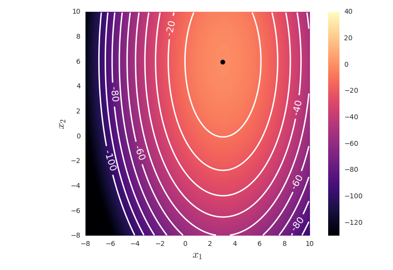
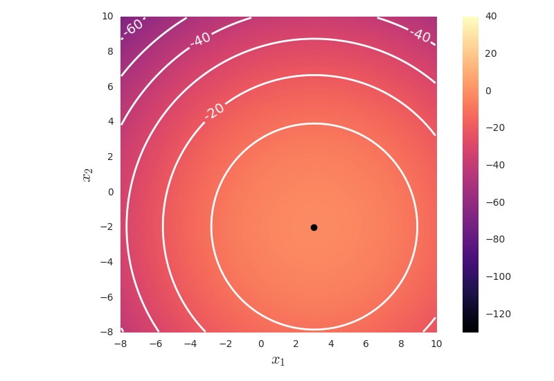
From this we can draw the contours of the covariance matrices

Figure 1.1 Contours of the covariance matrices plotted on top of the graph of the unnormalized log posterior function of the respective classes. Class 1 is depicted to the left and class 2 to the right.

b)

If we take the log posterior as the discrimination function (where we assume equal prior probability, and have removed the independent constants),

$d_c(x) = -\frac{1}{2}\log(\det(\Sigma_c)) - \frac{1}{2}(x - \mu_c)^\intercal \Sigma_c^{-1}(x - \mu_c)$

we get, for class 1

$\begin{align} d_1(x) &= -\frac{1}{2}\log(1) - \frac{1}{2} [x_1 - 3, x_2 - 6] \left[ \begin{array}{c} 2(x_1 - 3) \\ 1/2(x_2 - 6) \end{array} \right] \\[0.5ex] &= -\frac{1}{2}\left[2(x_1 - 3)^2 + \frac{1}{2}(x_2 - 6)^2 \right] \\[0.5ex] &= -x_1^2 + 6x_1 - \frac{1}{4}x_2^2 + 3x_2 - 18, \end{align}$

and for class 2

$\begin{align} d_2(x) &= -\frac{1}{2}\log(4) - \frac{1}{2} [x_1 - 3, x_2 + 2] \left[ \begin{array}{c} 1/2(x_1 - 3) \\ 1/2(x_2 + 2) \end{array} \right] \\[0.5ex] &= -\frac{1}{4}\left[2\log(4) + (x_1 - 3)^2 + (x_2 + 2)^2 \right] \\[0.5ex] &= -\frac{1}{4}x_1^2 + \frac{3}{2}x_1 - \frac{1}{4}x_2^2 - x_2 - \frac{13}{4} - \log(2). \end{align}$

We get the equation for the decision boundary by setting $d_1(x) = d_2(x)$ , which results in

$\begin{align} x_2 &= \frac{1}{4}\left[x_1^2 - 6x_1 + 18 -\frac{1}{4}x_1^2 + \frac{3}{2}x_1 - \frac{13}{4} - \log(2)\right] \\[0.5ex] &= \frac{3}{16}x_1^2 - \frac{9}{8}x_1 + \frac{59}{16} - \frac{1}{4}\log(2). \end{align}$

c)

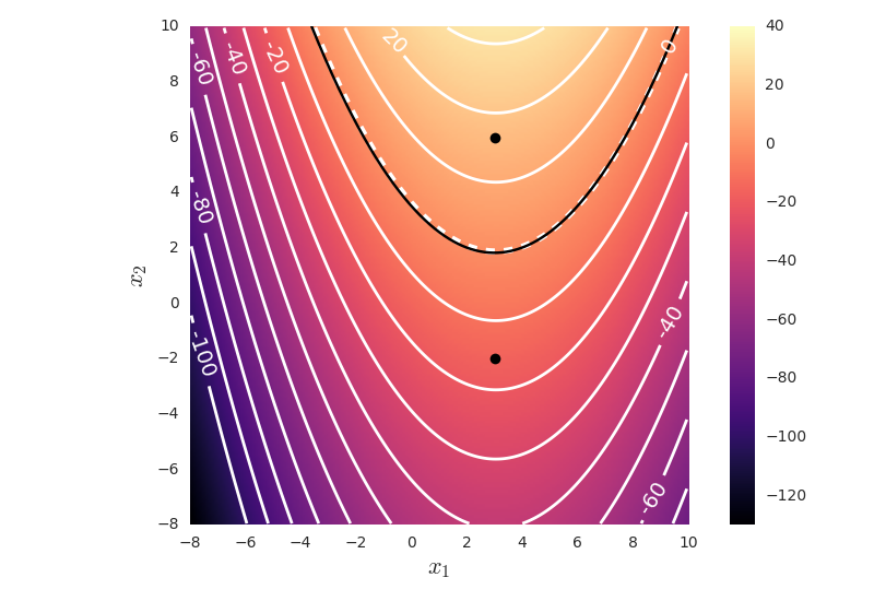
Here, we show the graph of the decision boundary on top of the graph of the difference between the unnormalized log posteriors of the classes. We see that all points where the graph is zero is on the decision boundary, all points with a positive difference value belongs to class 1, and all points with a negative difference value belongs to class 2.

Figure 1.2 Contours (white), and the graph of the difference between the unnormalized log posterior of class 2 and the posterior of class 1. Plotted on top in black, is the graph of the decision boundary.

d)

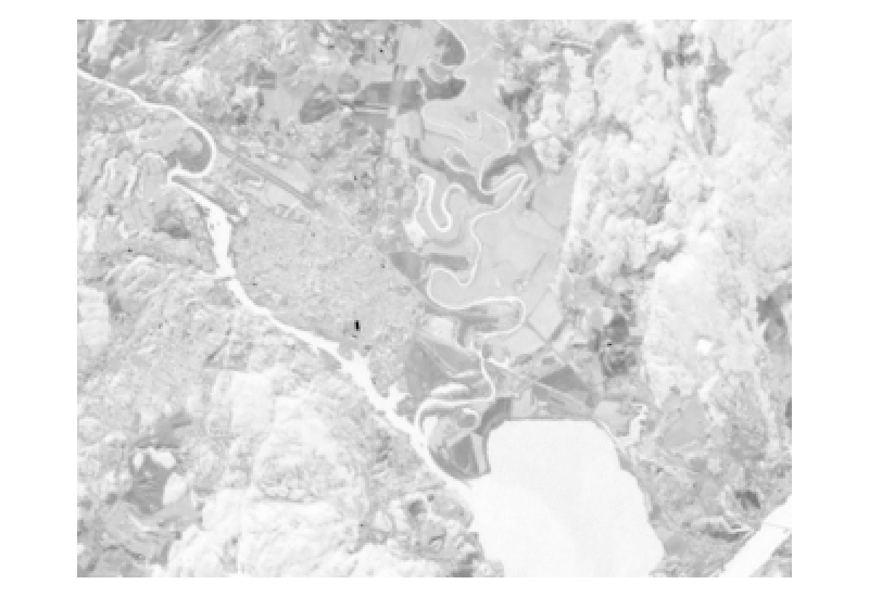
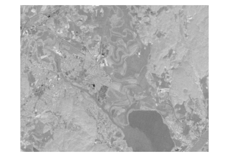
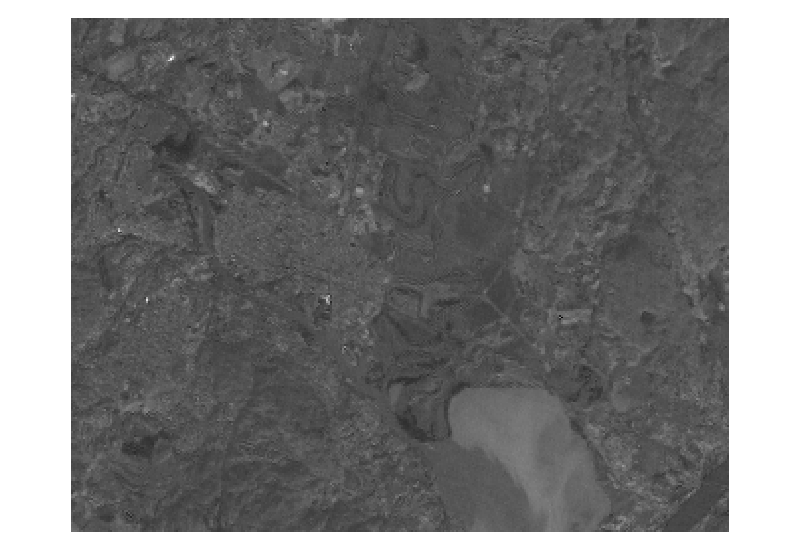
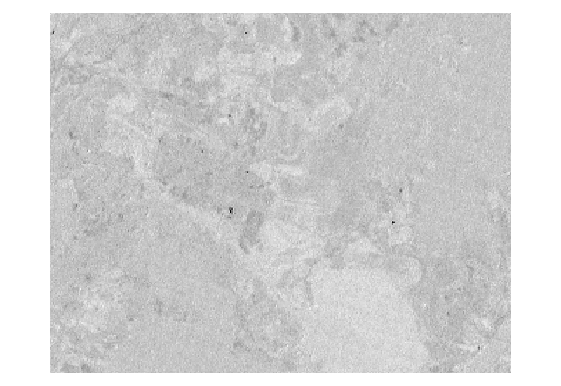
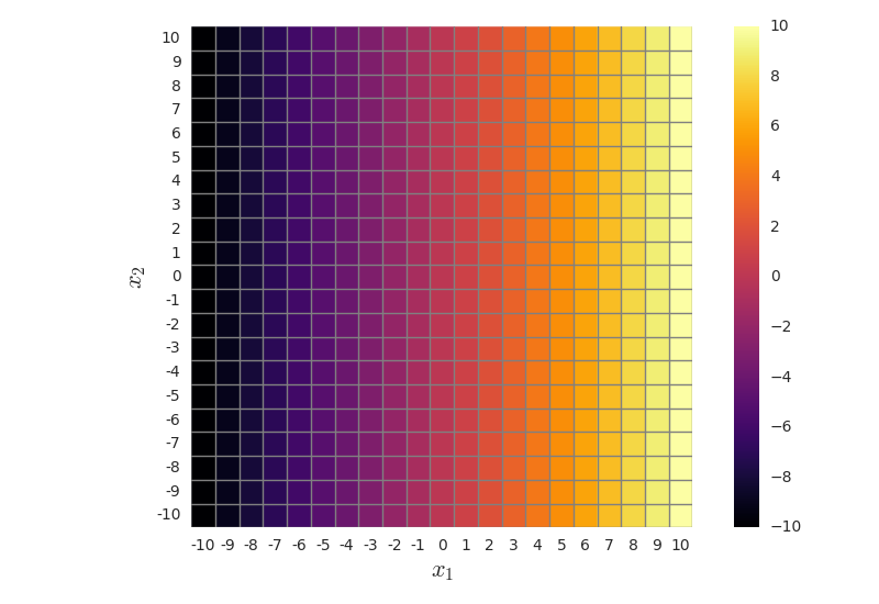
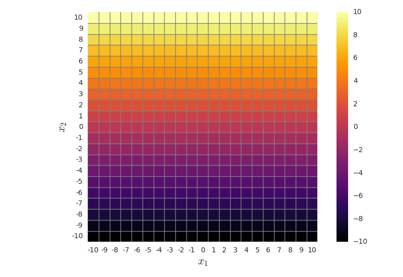
The feature images looks like this

Figure 1.3 Feature image 1 (left) and 2 (right).

e)

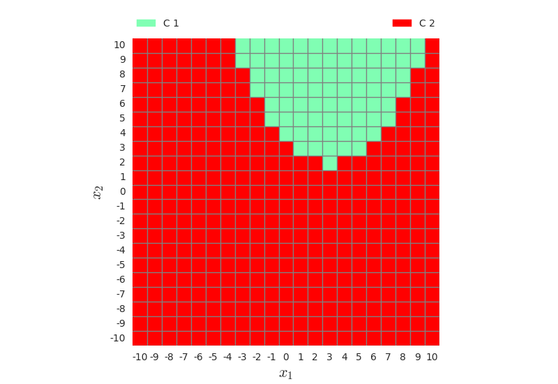
Figure 1.4 shows the classification, both done with tha analytical decision boundary (left), and the result from the multivariate gaussian classifier from week 7 (right). They are equal, and correspond well to the shape of the decision boundary.

Figure 1.4.

Task 2 - Principal Component Analysis

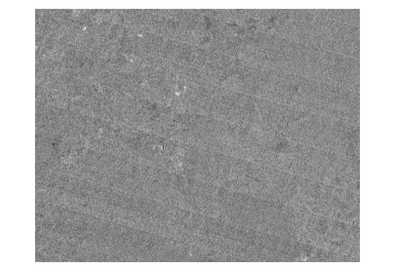
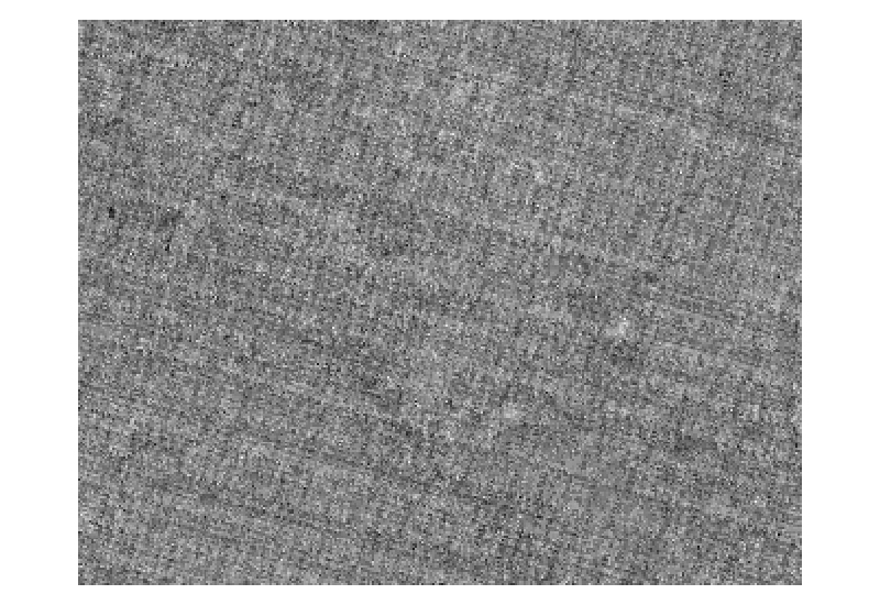
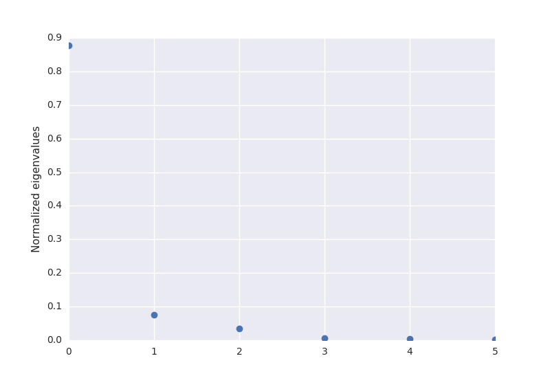
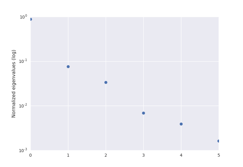
The 6 principal component images of the Kjeller landsat images.

Figure 1.1 PC 1 (left) and 2 (right).

Figure 1.2 PC 3 (left) and 4 (right).

Figure 1.3 PC 5 (left) and 6 (right).

Figure 1.4 Eigenvalues of the covariance matrix in decreasing order.

Figure 1.5 Class separation with the two first principal components.