Task 1

We have several design options for detecting gaps in lines, one such set could be

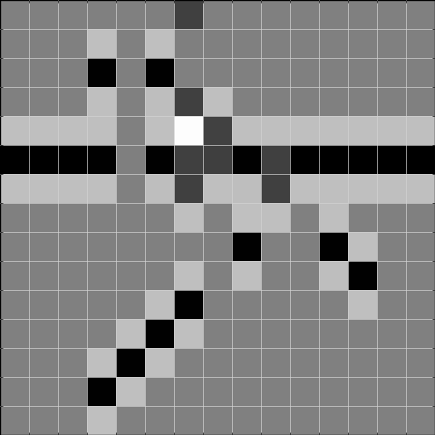
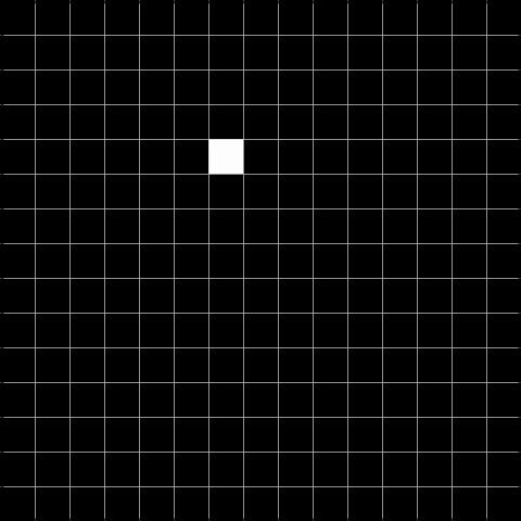
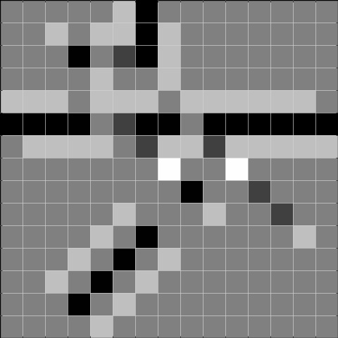
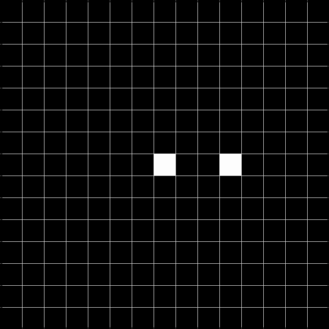
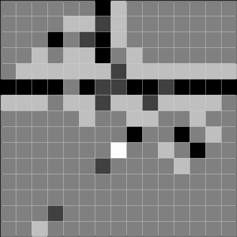
We can use these to detect gaps in horizontal, vertical, diagonal, and antidiagonal lines, respectively. We illustrate this by the dummy image shown in Figure 1.1.

Figure 1.1 Dummy image of lines with gaps.

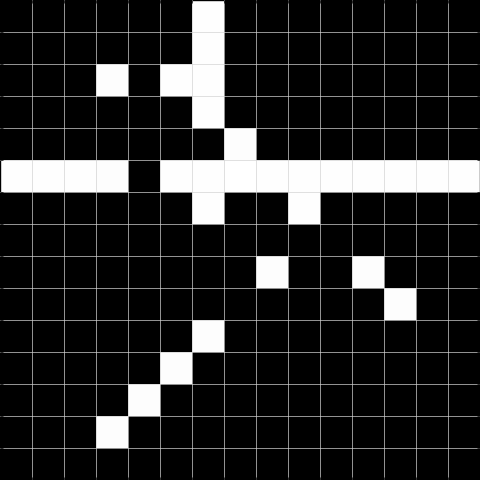
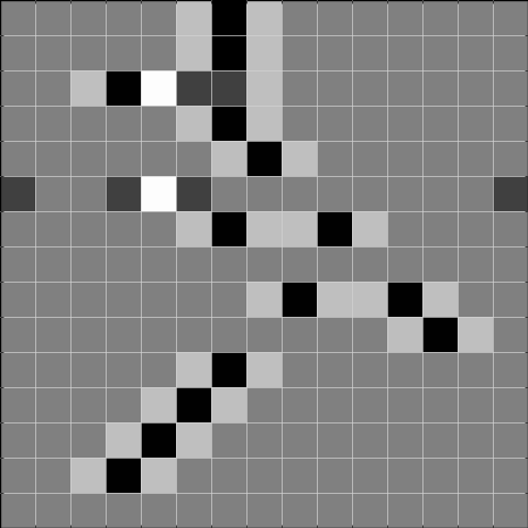
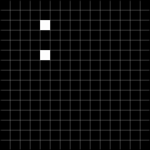
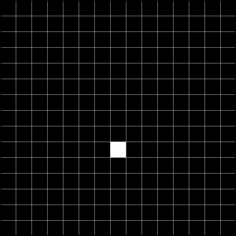
Below, we show the results after convolving the above image with the respective filters. The result to the left is the result of the convolution, and the result to the right is thresholded at 2, and can be used to detect the gaps.

Figure 1.2 Horizontal filter.

Figure 1.3 Vertical filter.

Figure 1.4 Diagonal filter.

Figure 1.5 Anti-diagonal filter.

Task 2

The image in problem 10.36 has a number of objects that are brighter than the background. We are given the information that the mean intensity of the backgroud is 60, while the mean intensity of the objects are 170 on a [0 255] scale.

We follow the procedure explained in section 10.4.1 in G&W on region-based segmentation. First, we choose to use foreground-seeds of 170, then use 8-connectivecty to “grow” our regions iteratively if the neighbouring pixel is for example larger than 115.

1. Threshold the image at 170 to create a seed image of the foreground.
2. For every connected foreground region, add a pixel to this region if:
   • The new pixel has gray level above 115
   • The new pixel is connected (with 8 connectivity) to the region.
3. Continue from 2. until the regions stop growing.

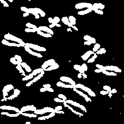
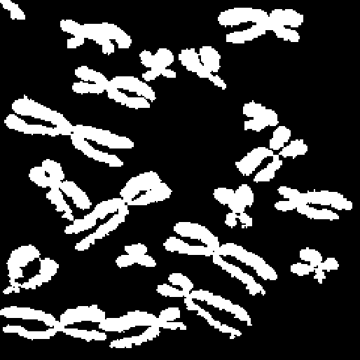
As an example, I have used region growing on the image shown in Figure 2.1 (I could not find the image used in the book).

Figure 2.1 Image of some chromosomes.

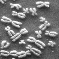
If we try a simple thresholding by Otsu, we get the result shown in Figure 2.2. We see that we also include some bright spots that we do not want. Note that there are probably simpler and/or better methods to segment this particular image, but it gives a simple illustration of the region growing.

Figure 2.2 Otsu binarization of image in Figure 2.1.

Figure 2.2 Gray level intensity distribution of image in Figure 2.1.

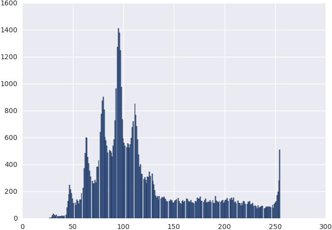
The gray level intensity distribution is shown in Figure 2.2, and from it, we choose the seed level to be 240, and the proposed region threshold to be at 150

Figure 2.3 Image thresholded at graylevel 240 (left) and 150 (right).

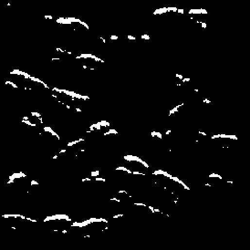
Using region growing of the seed image until convergence yields the final result shown in Figure 2.4.

Figure 2.4 Final segmentation using region growing from seed.

Task 3

The image we are to segment look like this.

Figure 3.1 Binary image.

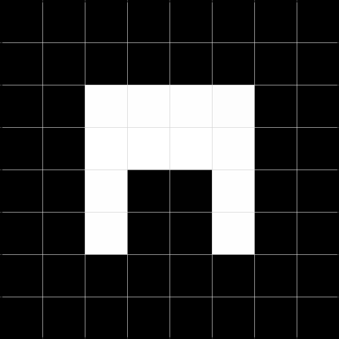
Splitting each quadrant not satisfying the criteria that every value in the region needs to be the same, results in a tree shown in Figure 3.2.

Figure 3.2 Quadtree.

With this, we can merge regions satisfying the criterion. In our case, this will result in a perfect segmentation.

Task 4

The one-dimensional intensity cross section given.

Figure 4.1 Data.

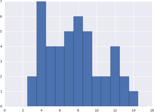
The step by step implementation would look something like this.

• Start with $n=1$. ($n = min(data) + 1$)
  • Two minimums: $[1, 2]$ and $[15]$
• Increase $n$ to $2$.
  • Basin $[15]$ will catch $14$
  • Current basins: $[1, 2]$ and $[14, 15]$
• Increase $n$ to $3$.
  • Basin $[1, 2]$ will catch $3$.
  • New minimum: $[10, 11]$
  • Basin $[14, 15]$ will catch $13$.
  • Current basins: $[1, 2, 3]$, $[10, 11]$ and $[13, 14, 15]$
• Increase $n$ to $4$.
  • Nothing happens.
• Increase $n$ to $5$.
  • New minimum: $[5, 6]$
  • New dam: $12$
  • Current basins: $[1, 2, 3]$, $[5, 6]$, $[10, 11]$ and $[13, 14, 15]$
  • Current dams: $12$
• Increase $n$ to $6$.
  • Basin $[5, 6]$ will catch $7$.
  • Basin $[10, 11]$ will catch $9$.
  • Current basins: $[1, 2, 3]$, $[5, 6, 7]$, $[9, 10, 11]$ and $[13, 14, 15]$
  • Current dams: $12$
• Increase $n$ to $7$.
  • New dam: $8$
  • Current basins: $[1, 2, 3]$, $[5, 6, 7]$, $[9, 10, 11]$ and $[13, 14, 15]$
  • Current dams: $8$ and $12$
• Increase $n$ to $8$.
  • New dam: $4$
  • Current basins: $[1, 2, 3]$, $[5, 6, 7]$, $[9, 10, 11]$ and $[13, 14, 15]$
  • Current dams: $4$, $8$ and $12$
• Finished! ($n = max(data)+1$)

Alternatively with a step prior to $n=1$ where a dam is created at each end of the function, i.e. at $n=1$ and $n=15$, to prevent the rising water from running off the ends. The remaining steps will be similar, only that the first and last basins won’t include $1$ and $15$, respectively.

Task 5

Figure 5.1 Original image of overlapping disks.

Figure 5.2 The istance transform to the left, and its negative counterpart to the right.

Figure 5.3 Result after watershed segmentation.

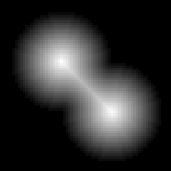
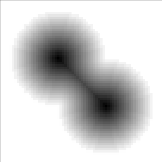
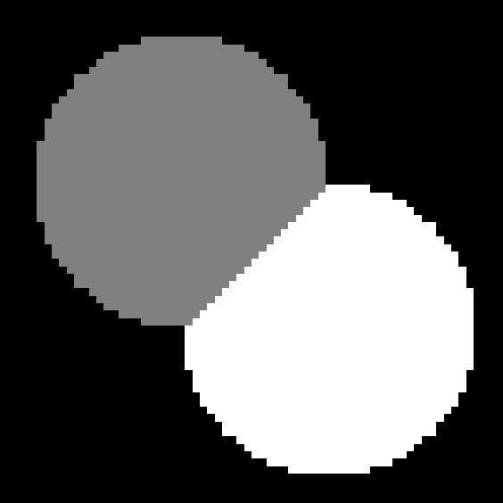
Task 6

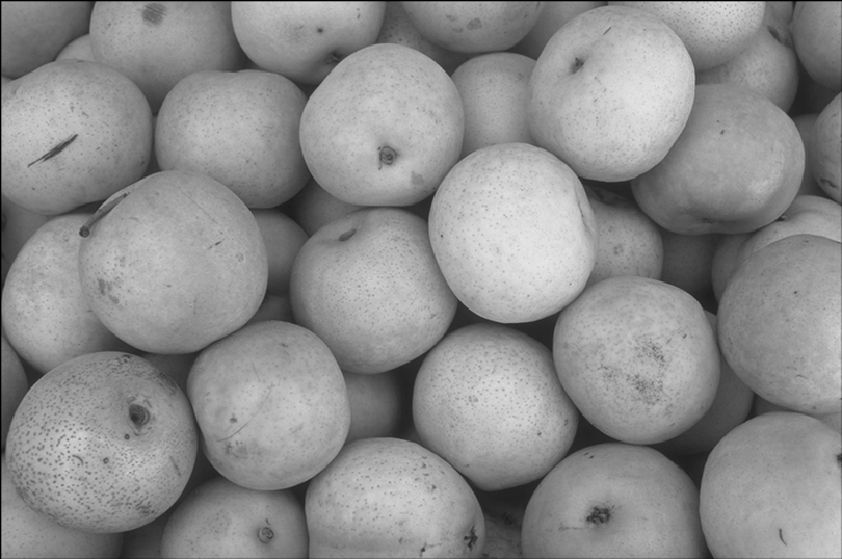
First, the grayscale version of the pear image.

Figure 6.1 Grayscale version of the pear image.

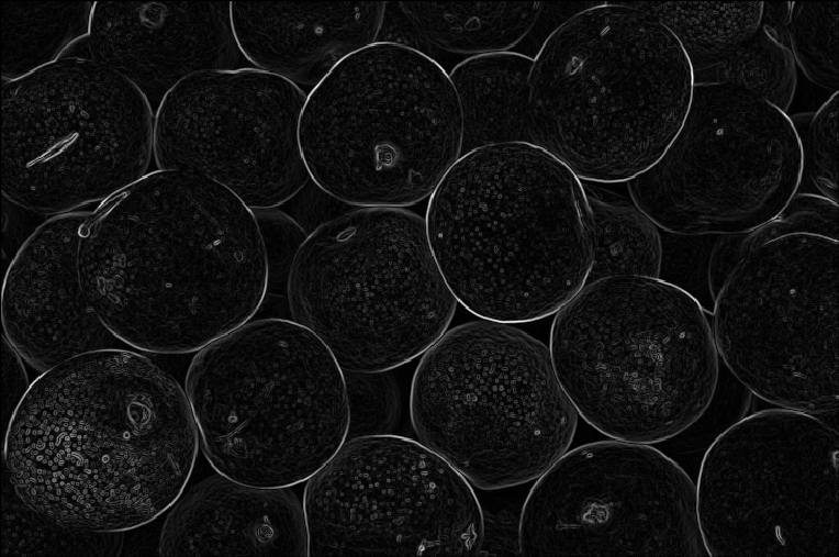
This gives quite nice gradients, but some additional things are needed before we can use it for watershed.

Figure 6.2 Gradient magnitude of pear image.

The simple morphological opening follows.

Figure 6.3 Morphological opening.

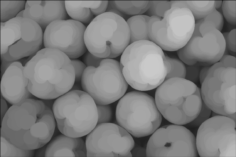
Which can be compared by the opening-by-reconstruction.

Figure 6.4 Opening-by-reconstruction.

Figure 6.5 Morphological closing of the opened image in Figure 6.3.

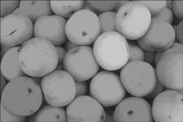
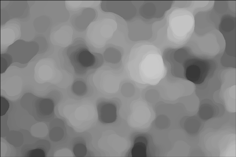
The one we are actually going to use is the closing-by-reconstruction of the opening-by-reconstruction.

Figure 6.6 Closing-by-reconstruction of the opened-by-reconstruction image in Figure 6.4.

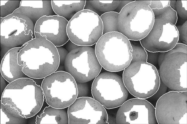
By using some maximum filters, we can find the regional maxima, and use them as sure foreground.

Figure 6.7 Regional maxima of the image in Figure 6.6.

Figure 6.8 Regional maxima superimposed on the original grayscale image.

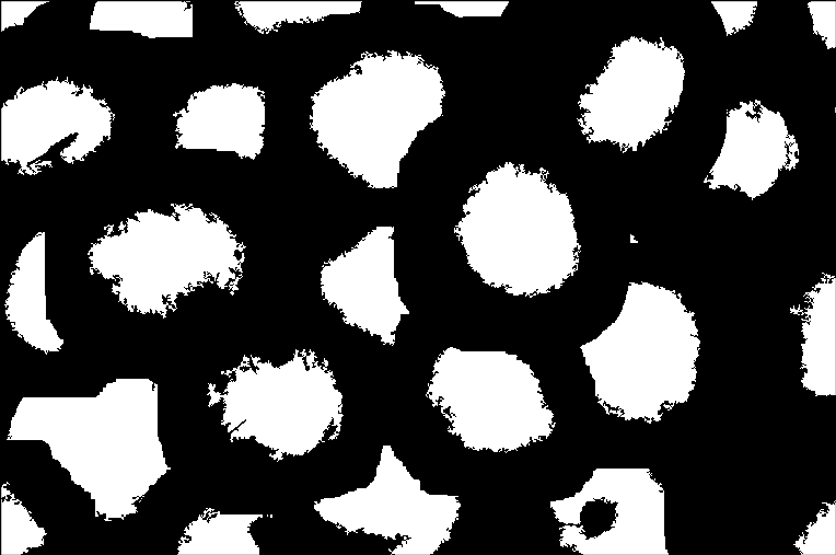
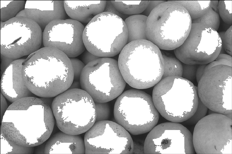
But first, we clean them a bit.

Figure 6.9 Modified foreground labeled and superimposed on the original grayscale image.

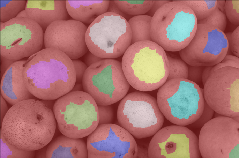
The backgorund in the thresholded image can be used as sure background.

Figure 6.10 Binary threshold of the image in Figure 6.6.

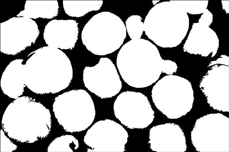
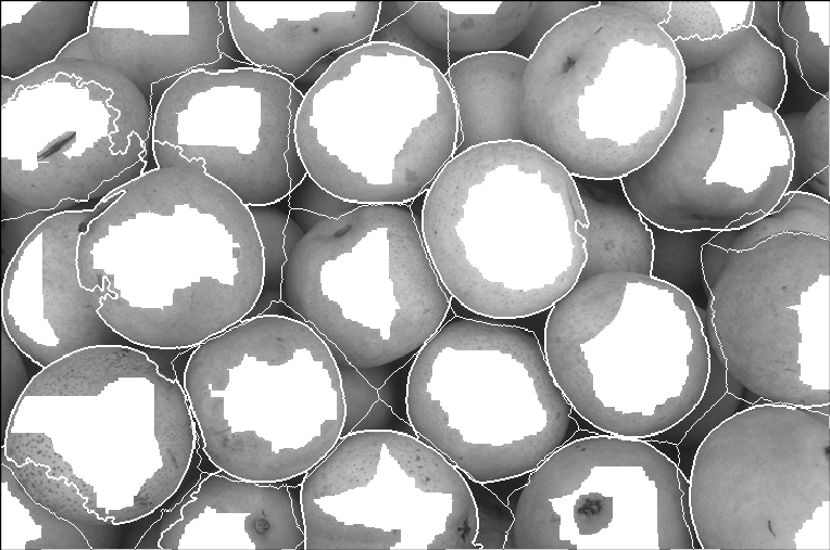
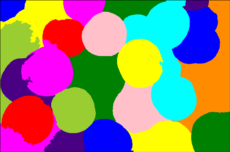
Finally, the watershed results.

Figure 6.11 Boundaries and foreground overlayed on the original.

Figure 6.12 Labels from the watershed segmentation.

Figure 6.13 Labels from the watershed segmentation overlayed the original grayscale image.

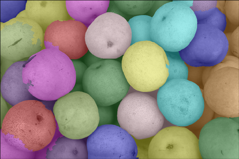
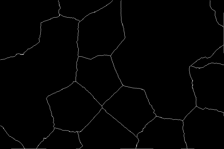
Now, if you did compute the SKIZ, you will see that it did not make any significant contribution. The results are as the one above, but with SKIZ.

Figure 6.14 Skeleton by influence zones (SKIZ) of the thresholded image.

Figure 6.15 Boundaries and foreground overlayed on the original.

Figure 6.16 Labels from the watershed segmentation.

Figure 6.17 Labels from the watershed segmentation overlayed the original grayscale image.

Task 7

Figure 7.1 Grayscale cell image.

Figure 7.2 Binary thresholded cell image.

Figure 7.3 Thresholded image where interior regions are filled.

Figure 7.4 Labeled regions from watershed.

Figure 7.5 Labeled regions from watershed overlayed the original image.