See the notes for reference both about the topic and the notation employed in this solution proposal.

Table of contents

• Task 1
• Task 2
• Task 3
• Task 4
• Task 5
• Task 6

Task 1 (Problem 11.1 in Gonzales and Woods)

1. Treating the chain code a circular, connected chain, it is obvious that every element corresponds to a unique starting point. Thus, by agreeing on the rule that the code should form an integer of minimum magnitude, we make the code invariant to the starting point. Note that this is somewhat arbitrary, and we could just as well use e.g. the configuration that forms the integer of maximum magnitude, as long as everyone agrees.

2. $$S([1,1,0,7,6,7,6,5,5,4,3,3,2,2]) = [0,7,6,7,6,5,5,4,3,3,2,2,1,1]$$

Task 2 (Problem 11.8 in Gonzales and Woods)

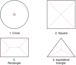
The medial axis or the skeleton of an object is defined as (see. section 11.1.7 in Gonzales and Woods).

For each point $p$ in a region $R$, we find its closest neighbor at the boundary $B$. If $p$ has more than one such neighbor, it is said to belong to the medial axis (skeleton) of $R$.

The concept of closest depends on our distance metric, and a below we employ the common Euclidean distance.

Figure 1: Skeletons of some objects. Note that the skeleton in the circle is just a single point.

Task 3 (Problem 11.9 in Gonzales and Woods)

Subtask 1

Apply Step 1 on all figures.

Figure 1

$\begin{array}{|c|c|c|} \hline 1 & 1 & 0 \\ \hline 1 & p & 0 \\ \hline 1 & 1 & 0 \\ \hline \end{array}$

a) $N(p) = 5 \quad \Rightarrow$ OK.

b) $T(p) = 1 \quad \Rightarrow$ OK.

c) $p_2 \cdot p_4 \cdot p_6 = 0 \quad \Rightarrow$ OK.

d) $p_4 \cdot p_6 \cdot p_8 = 0 \quad \Rightarrow$ OK.

Every condition is met, so flag this point.

Figure 2

$\begin{array}{|c|c|c|} \hline 0 & 0 & 0 \\ \hline 1 & p & 0 \\ \hline 0 & 0 & 0 \\ \hline \end{array}$

a) $N(p) = 1 \quad \Rightarrow$ not OK.

b) $T(p) = 1 \quad \Rightarrow$ OK.

c) $p_2 \cdot p_4 \cdot p_6 = 0 \quad \Rightarrow$ OK.

d) $p_4 \cdot p_6 \cdot p_8 = 0 \quad \Rightarrow$ OK.

Condition a) is not met, so keep this point.

Figure 3

$\begin{array}{|c|c|c|} \hline 0 & 1 & 0 \\ \hline 1 & p & 1 \\ \hline 0 & 1 & 0 \\ \hline \end{array}$

a) $N(p) = 4 \quad \Rightarrow$ OK.

b) $T(p) = 4 \quad \Rightarrow$ not OK.

c) $p_2 \cdot p_4 \cdot p_6 = 1 \quad \Rightarrow$ not OK.

d) $p_4 \cdot p_6 \cdot p_8 = 1 \quad \Rightarrow$ not OK.

Only condtion a) is met, so keep this point.

Figure 4

$\begin{array}{|c|c|c|} \hline 1 & 1 & 0 \\ \hline 0 & p & 1 \\ \hline 0 & 0 & 0 \\ \hline \end{array}$

a) $N(p) = 3 \quad \Rightarrow$ OK.

b) $T(p) = 2 \quad \Rightarrow$ not OK.

c) $p_2 \cdot p_4 \cdot p_6 = 0 \quad \Rightarrow$ OK.

d) $p_4 \cdot p_6 \cdot p_8 = 0 \quad \Rightarrow$ OK.

Condition b) is not met, so keep this point.

Subtask 2

Apply Step 2 on all figures.

Figure 1

$\begin{array}{|c|c|c|} \hline 1 & 1 & 0 \\ \hline 1 & p & 0 \\ \hline 1 & 1 & 0 \\ \hline \end{array}$

a) $N(p) = 5 \quad \Rightarrow$ OK.

b) $T(p) = 1 \quad \Rightarrow$ OK.

c) $p_2 \cdot p_4 \cdot p_8 = 0 \quad \Rightarrow$ OK.

d) $p_2 \cdot p_6 \cdot p_8 = 1 \quad \Rightarrow$ not OK.

Condition d) is not met, so keep this point.

Figure 2

$\begin{array}{|c|c|c|} \hline 0 & 0 & 0 \\ \hline 1 & p & 0 \\ \hline 0 & 0 & 0 \\ \hline \end{array}$

a) $N(p) = 1 \quad \Rightarrow$ not OK.

b) $T(p) = 1 \quad \Rightarrow$ OK.

c) $p_2 \cdot p_4 \cdot p_8 = 0 \quad \Rightarrow$ OK.

d) $p_2 \cdot p_6 \cdot p_8 = 0 \quad \Rightarrow$ OK.

Condition a) is not met, so keep this point.

Figure 3

$\begin{array}{|c|c|c|} \hline 0 & 1 & 0 \\ \hline 1 & p & 1 \\ \hline 0 & 1 & 0 \\ \hline \end{array}$

a) $N(p) = 4 \quad \Rightarrow$ OK.

b) $T(p) = 4 \quad \Rightarrow$ not OK.

c) $p_2 \cdot p_4 \cdot p_8 = 1 \quad \Rightarrow$ not OK.

d) $p_2 \cdot p_6 \cdot p_8 = 1 \quad \Rightarrow$ not OK.

Only condtion a) is met, so keep this point.

Figure 4

$\begin{array}{|c|c|c|} \hline 1 & 1 & 0 \\ \hline 0 & p & 1 \\ \hline 0 & 0 & 0 \\ \hline \end{array}$

a) $N(p) = 3 \quad \Rightarrow$ OK.

b) $T(p) = 2 \quad \Rightarrow$ not OK.

c) $p_2 \cdot p_4 \cdot p_8 = 0 \quad \Rightarrow$ OK.

d) $p_2 \cdot p_6 \cdot p_8 = 0 \quad \Rightarrow$ OK.

Condition b) is not met, so keep this point.

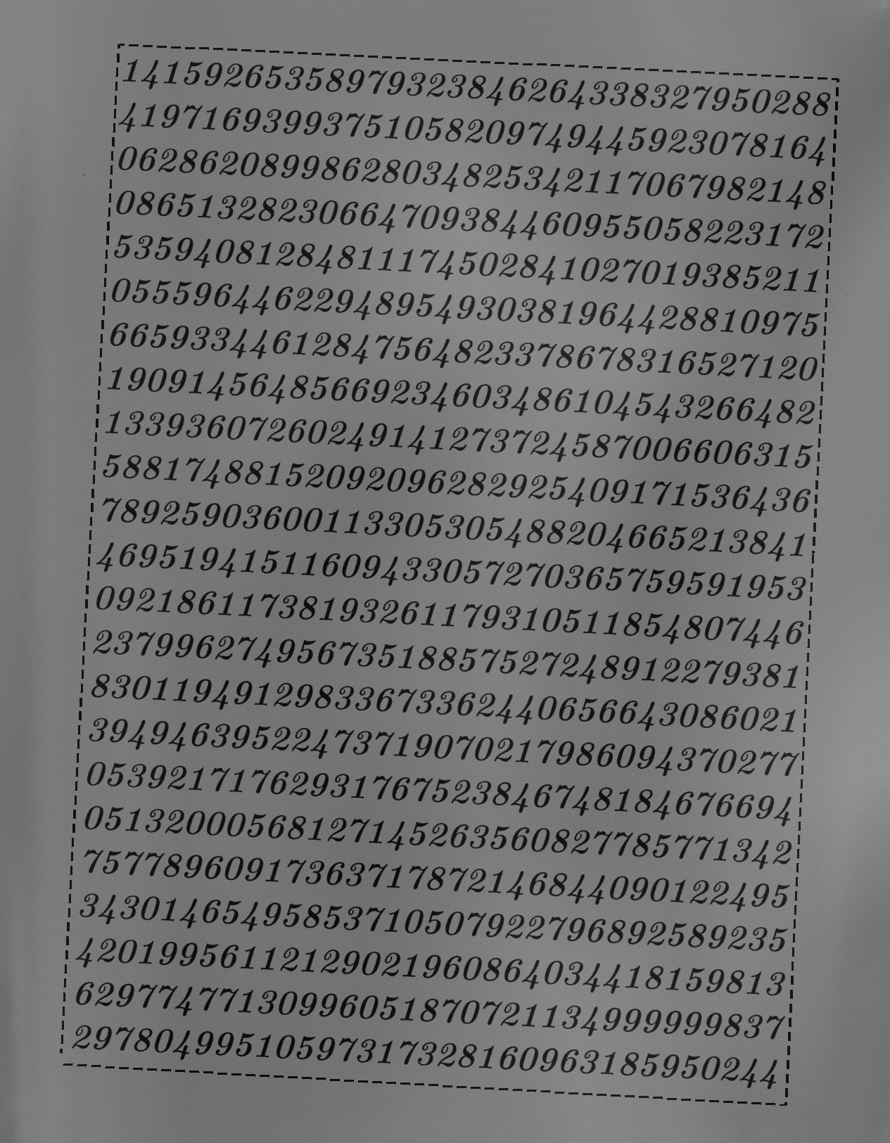
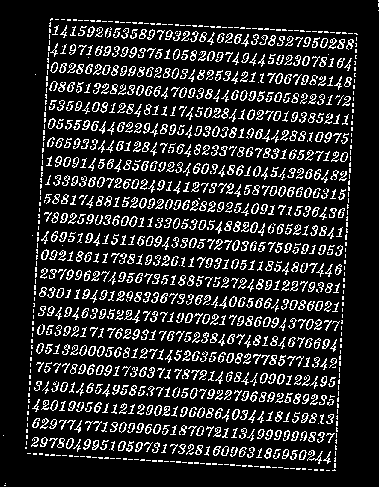
Task 4 - Create region objects using Python

In this task, we will find connected regions in an image and remove unwanted objects based on information about these regions. The full source code, named inf4300_h16_ex04_t04.py is can be found here.

Step 0 - Some necessary imports

import numpy as np
import matplotlib.pyplot as plt
import cv2
from skimage.color import label2rgb

Step 1 - Read the image

Read the image as a grayscale image, but remember to cast it to float. The reason for this is that some of the operations we are performing later (like subtraction of images) are going to give values outside the [0, 255] range. If we had kept an unsigned integer type for our image, unexpected things could occur (and we would not necessary be warned about it).

image = cv2.imread(image_file, cv2.IMREAD_GRAYSCALE)
image = image.astype(np.float32)

Figure 2: Grayscale 'tall_noise10_backgr.png'.

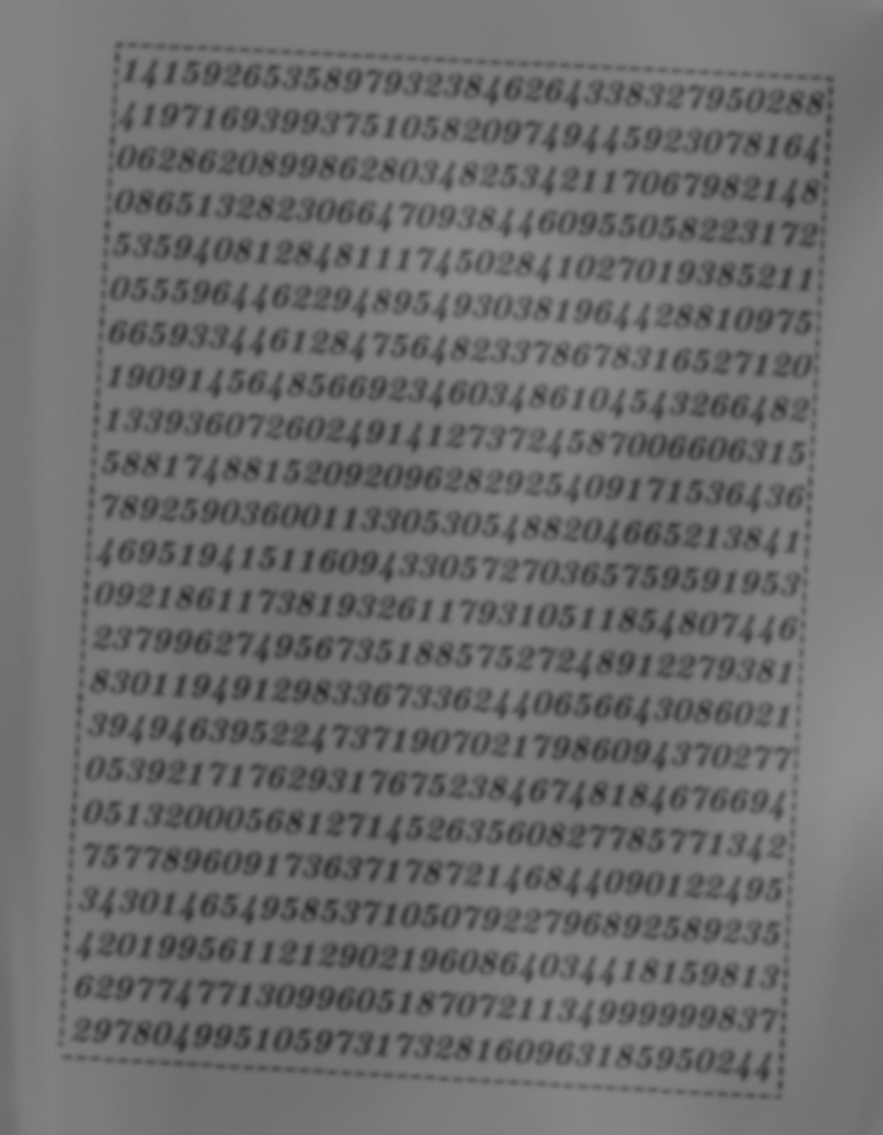
Step 2 - Remove high-frequency noise

We do this by applying some blurring filter (low-pass filtering, letting the low frequencies through, stopping high frequencies). Here are some different blur functions in openCV you can try for both step 2 and step 3.

ksize = 5 # Some odd integer
blurred_image = cv2.blur(image, (ksize, ksize)) # Mean blur
blurred_image = cv2.GaussianBlur(image, (ksize, ksize), 0)
blurred_image = cv2.medianBlur(image, ksize)
blurred_image = cv2.biliteralFilter(imag, 9, 75, 75) # Read the docs

In this proposal, I used a Gaussian filter with kernel size 5

nr_image = cv2.GaussianBlur(image, (5, 5), 0)

Figure 3: Image blurred with a Gaussian filter to remove noise.

Step 3 - Create background image

I found that using Gaussian filtering again worked okay, albeit with a larger kernel size.

background = cv2.GaussianBlur(nr_image, (21, 21), 0)

Figure 4: Background image, obtained by yet another blurring.

Step 4 - Remove background

This subtraction will center the values around zero, so we rescale the graylevels back to the [0, 255] range, and cast it back to int.

br_image = nr_image - background
br_image = 255*(br_image - np.min(br_image)) / (np.max(br_image) - np.min(br_image))
br_image = br_image.astype(np.uint8)

Figure 5: Blurred image minus the background.

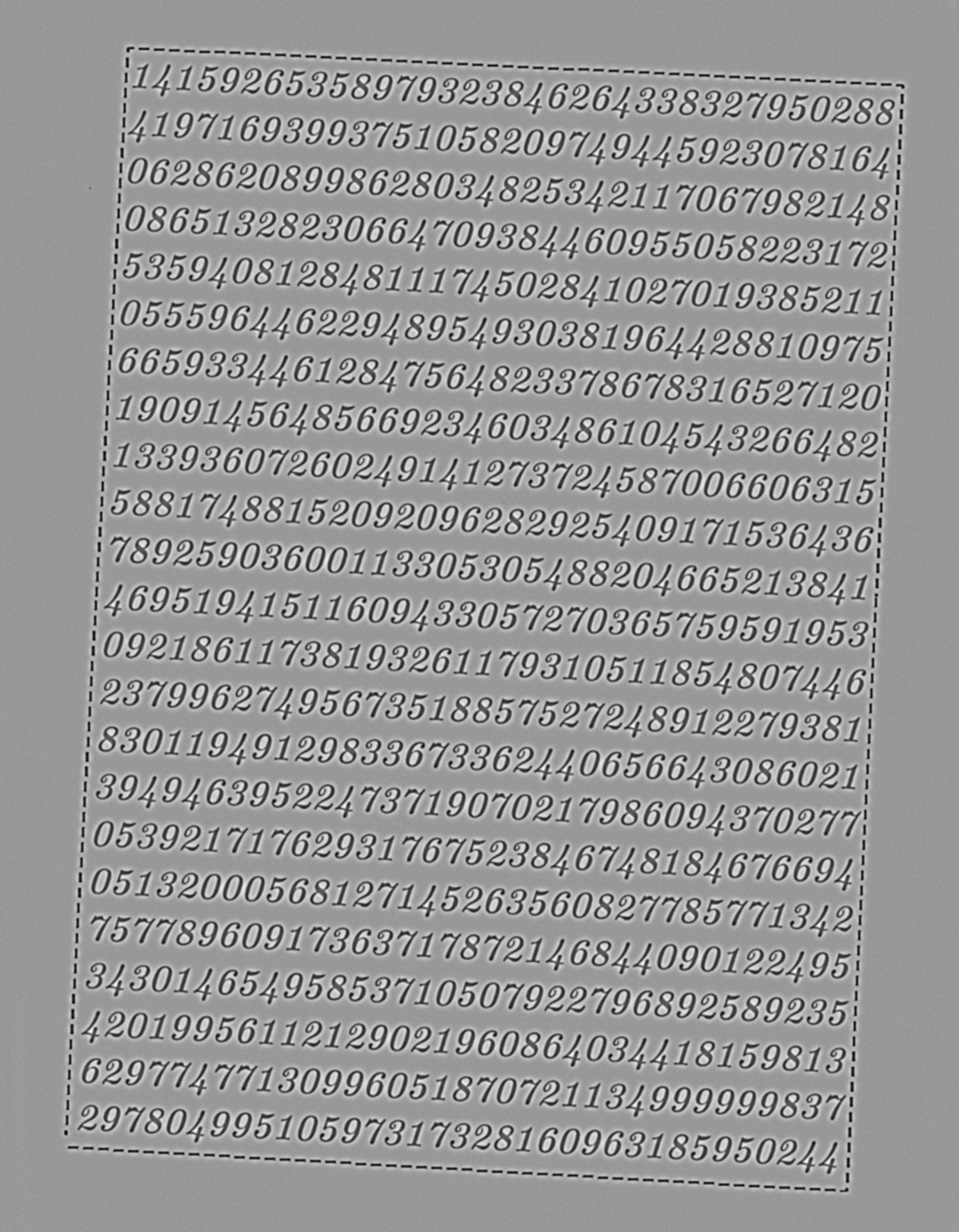
Step 5 - Threshold the image on intensity using a global threshold

Unless you are doing some automatic thresholding, it would be wise to see a distribution of the graylevels before deciding for a threshold.

Figure 6: Histogram of the graylevels in the image from Figure 5.

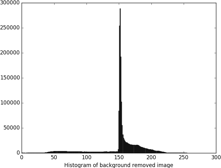
Here, we see that there is a large spike in the middle, which is recognizable as the majority of the background. Therefore we set the threshold right below this. As the interesting regions are darker than the background, we choose to “keep” the pixels with levels below this threshold. We cast the image from bool to int for later use. Note that now, the background is black, while the interesting regions are white.

threshold = 149
thr_image = (br_image < threshold).astype(np.uint8)

Figure 7: Result after manually thresholding by graylevel intensity.

Step 7 - Compute region objects and labels

Here, we are using a handy function that labels all connected regions with a unique label, and in addition, collects some useful information about the regions.

connectivity = 4
output = cv2.connectedComponentsWithStats(thr_image.astype(np.uint8),
                                          connectivity,
                                          cv2.CV_32S)
num_labels = output[0]
label_image = output[1] # Image with a unique label for each connected region
stats = output[2]
centroids = output[3] # Centroid indices for each connected region

Most interesting to us is the label_image and stats. The label_image is an array of the same shape as the input array, where each connected region has has a unique label.

Figure 8: Label image represented in the rgb colorspace.

The stats output is an array, where for each connected component, the following information is computed

• stats[:, 0]: The leftmost coordinate which is the inclusive start of the bounding box in the horizontal direction.
• stats[:, 1]: The topmost coordinate which is the inclusive start of the bounding box in the vertical direction.
• stats[:, 2]: The horizontal size of the bounding box.
• stats[:, 3]: The vertical size of the bounding box.
• stats[:, 4]: The total area (in pixels) of the connected component.

Step 8 - Use information about region to remove noise and the frame

First, we plot the histogram based on region area. Note that we slice away the first index since this correspond to the background label (and has thus a quite huge area compared to the other regions, which will mask our results).

region_area = stats[1:, 4]

Figure 9: Histogram of region area.

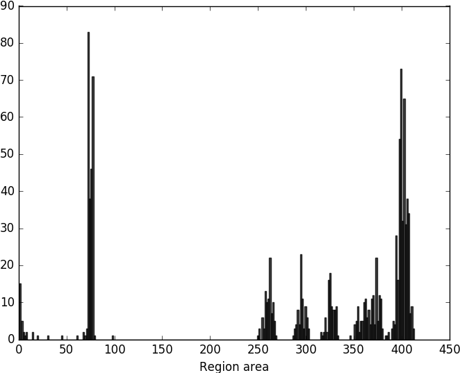
We can also create a scatterplot of the region area and the bounding box area, this will give us yet another view of the area distribution. It could be argued that the information added by the bounding box area is redundant, but the idea that you can use a scatterplot to visualize distributions of different qualities is instructive.

bbox_area = stats[1:, 2] * stats[1:, 3]

Figure 10: Scatterplot of region area and bounding-box area.

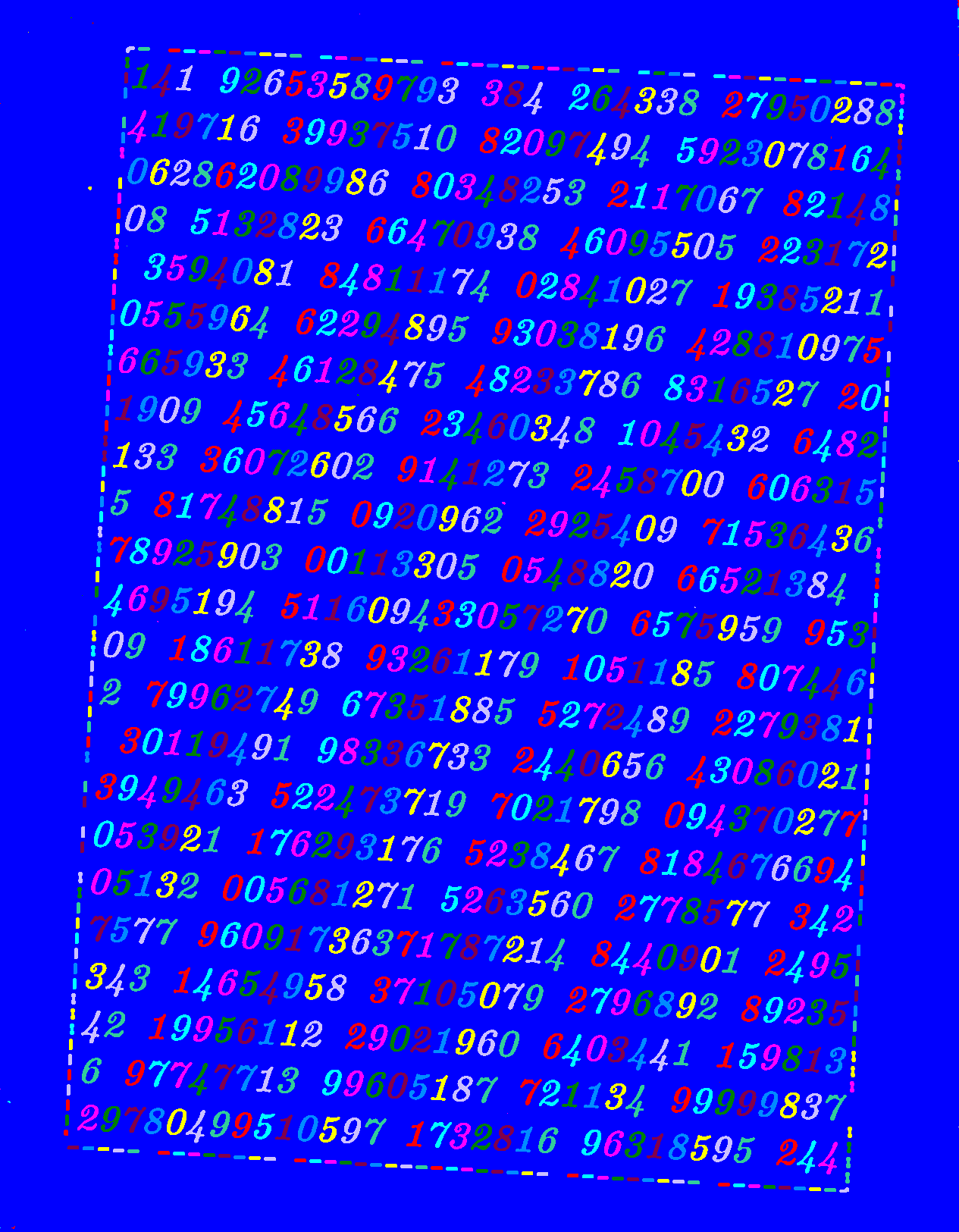
Finally, we use the gathered information to highlight different labels. Here we only use region area information.

region_area = stats[:, 4]
lower_threshold = 200
upper_threshold = 450
keep_labels = np.where(np.logical_and(stats[:, 4] > lower_threshold,
                                      stats[:, 4] < upper_threshold))
keep_label_image = np.in1d(label_image, keep_labels).reshape(label_image.shape)
ra_thr_image = np.copy(thr_image)
ra_thr_image[keep_label_image] = 255
ra_thr_image[keep_label_image == False] = 0

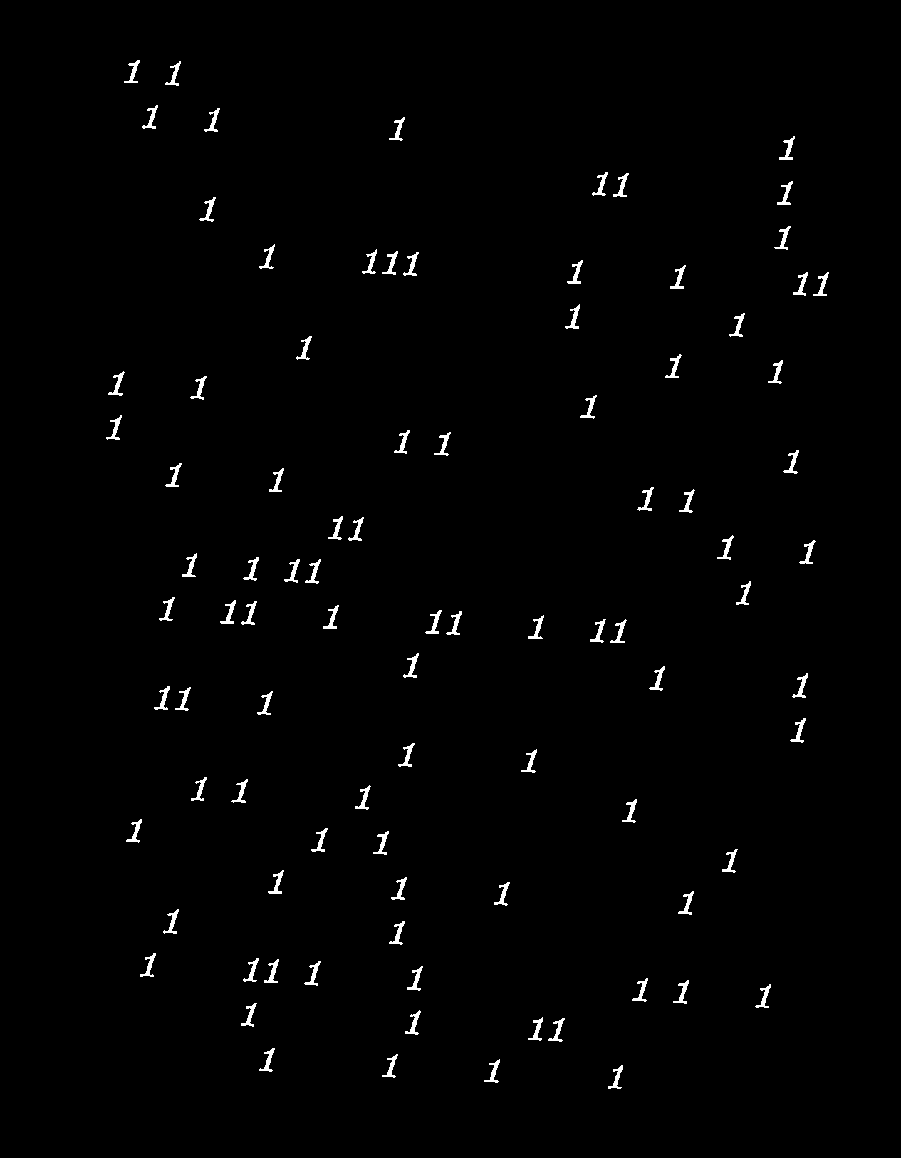
With the region area, we can easily filter out the noisy particles, and also discriminate between the frame and the numbers.

Figure 11: Left: Frame only, area interval: (50, 100). Right: Numbers only, area interval: (200, 450).

It is also easy to find ones, and the sevens,

Figure 12: Left: Number 1, area interval: (245, 275). Right: Number 7, area interval: (275, 310).

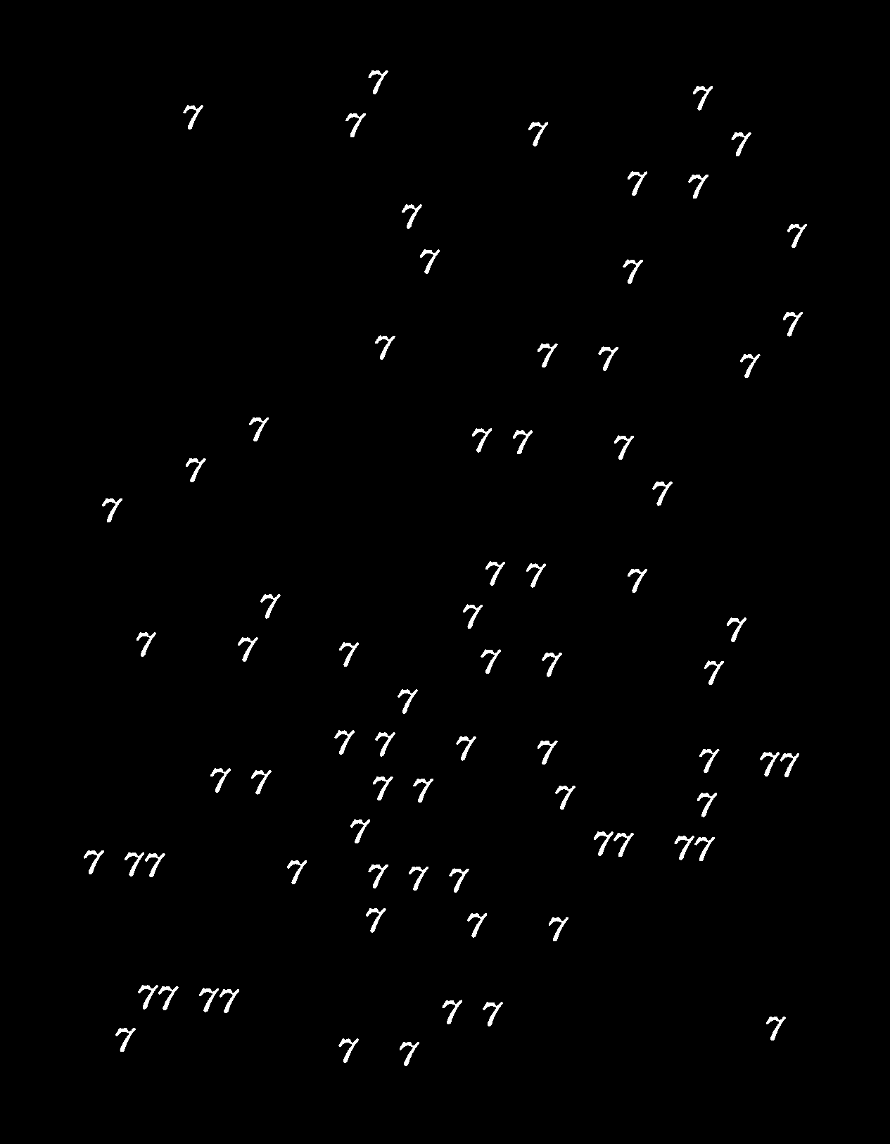
and even the fours. However, the rest seems a bit challenging using only region area information. In the right image are all threes and fives, but also one nine.

Figure 13: Left: Number 4, area interval: (310, 340). Right: Aarea interval: (340, 388).

The final group in the histogram contains all the eights, zeros, twos and rest of the nines.

Figure 14: Area interval: (388, 450).

Task 5 - Exercise 1 from 2011 exam: chain codes

1. Starting from the lower left pixel

   $$c_8 = (1,1,7,7,4,3,5,4)$$

2. We can apply minimum circular shift to make the chain code invariant to starting position. Applied on the code obtained from starting at the lower left pixel of the object “$\Lambda$”

   $$\begin{align} c_8 &= (1,1,7,7,4,3,5,4), \\ S(c_8) &= (1,1,7,7,4,3,5,4). \end{align}$$

   And then, the same applied to the chain code obtained from starting at the top pixel of the object “$\Lambda$”

   $$\begin{align} c_8 &= (7,7,4,3,5,4,1,1), \\ S(c_8) &= (1,1,7,7,4,3,5,4). \end{align}$$

3. Relative chain code is already rotation invariant, so we only need to apply starting point normalization. Starting at the upper left pixel of the rotated object “V” (remembering to substitute the first number since this is relative chain code), and using 0 as the forward direction, yields

   $$\begin{align} c_8 &= (5,7,2,7,5,0,6,0), \\ S(c_8) &= (0,5,7,2,7,5,0,6). \end{align}$$

   We can check this by applying rotation normalization to the code obtained from the $\Lambda$-shaped object.

   $$\begin{align} R(S(c_8)) &= (0,6,0,5,7,2,7,5), \\ S(R(S(c_8))) &= (0,5,7,2,7,5,0,6). \end{align}$$

Task 6 - Exercise 2 from 2012 exam: chain codes

1. Starting from the upper left pixel (at [0, 1])

   $$c_8 = (0,6,,7,0,6,4,5,4,3,2,1,2).$$

2. Applying minimum circular shift will make the code invariant to starting position (also apply rotation normalization for reference in step 3.)

   $$\begin{align} c_8 &= (0,6,7,0,6,4,5,4,3,2,1,2), \\ S(c_8) &= (0,6,4,5,4,3,2,1,2,0,6,7), \\ R(S(c_8)) &= (6,6,1,7,7,7,7,1,6,6,1,1), \\ S(R(S(c_8))) &= (1,1,6,6,1,7,7,7,7,1,6,6). \end{align}$$

   Compare with the result obtained when starting from the lower right pixel (at position [4, 2]).

   $$\begin{align} c_8 &= (4,3,2,1,2,0,6,7,0,6,4,5), \\ S(c_8) &= (0,6,4,5,4,3,2,1,2,0,6,7), \\ R(S(c_8)) &= (6,6,1,7,7,7,7,1,6,6,1,1), \\ S(R(S(c_8))) &= (1,1,6,6,1,7,7,7,7,1,6,6). \end{align}$$

3. Applying first difference on the chain code, and then normalizing it for starting point will make the code rotation invariant.

   Rotated object, starting from upper left (at [0, 2])

   $$\begin{align} c_8 &= (0,6,7,6,5,4,3,4,2,0,1,2), \\ R(c_8) &= (6,1,7,7,7,7,1,6,6,1,1,6), \\ S(R(c_8)) &= (1,1,6,6,1,7,7,7,7,1,6,6). \end{align}$$

   Rotated object, starting from lower right (at [4, 3])

   $$\begin{align} c_8 &= (4,3,4,2,0,1,2,0,6,7,6,5), \\ R(c_8) &= (7,1,6,6,1,1,6,6,1,7,7,7), \\ S(R(c_8)) &= (1,1,6,6,1,7,7,7,7,1,6,6). \end{align}$$

   Compare it to the results obtaned in step 2. to see that they are equal.