Solution proposal - exercise 7

Task 1

We are asked to implement a multivariate Gaussian classifier, and use it to classify images using a multiple of different features. I will only list the results in the following, but the source for obtaining these results is available here, and all images used are available here.

Figure 1.1 Feature images `tm1.png` (left) and `tm2.png` (right).

Figure 1.2 Feature images `tm3.png` (left) and `tm4.png` (right).

Figure 1.3 Feature images `tm5.png` (left) and `tm6.png` (right).

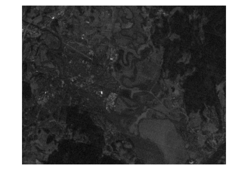
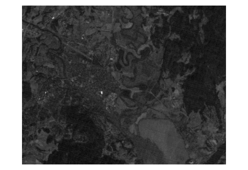
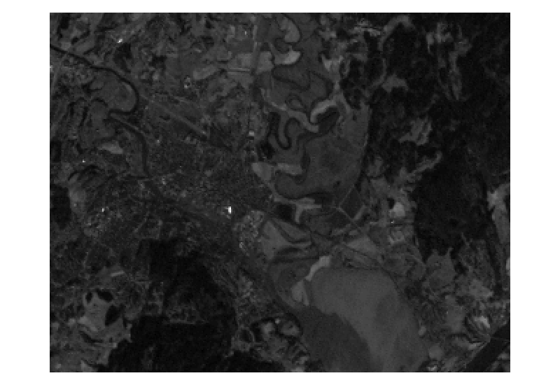
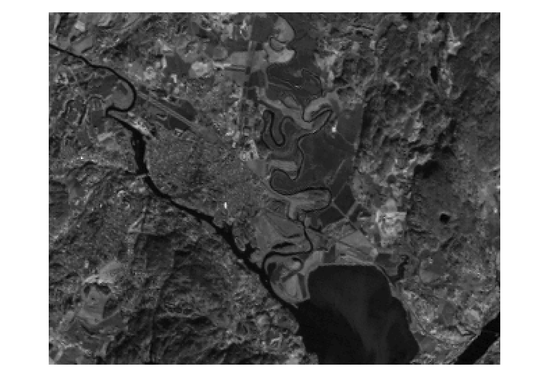
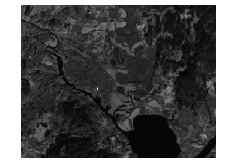
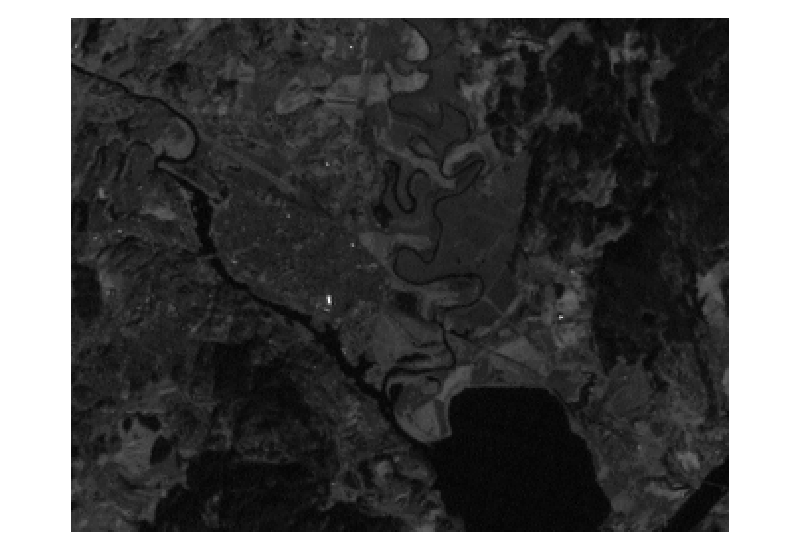
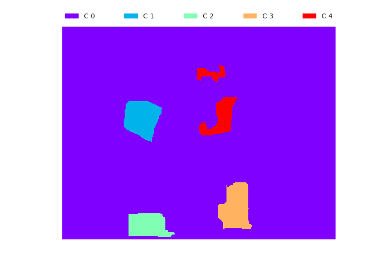
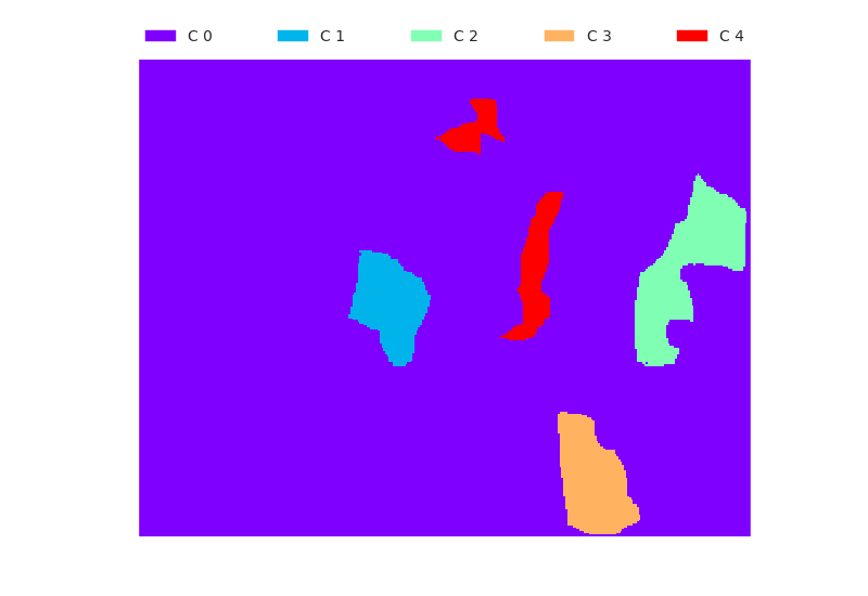
The following masks where used to obtain training features, and test features, respectively.

Figure 1.4 Train mask (left), and test mask (right).

One single feature image

Here we are only using feature image tm1.png.

Figure 1.5 Posterior images.

Figure 1.6 Classification result.

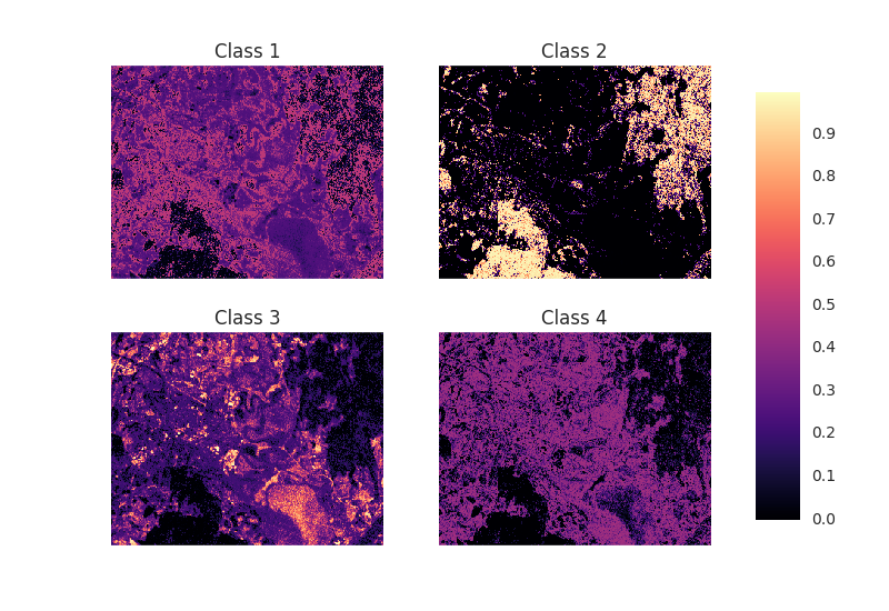
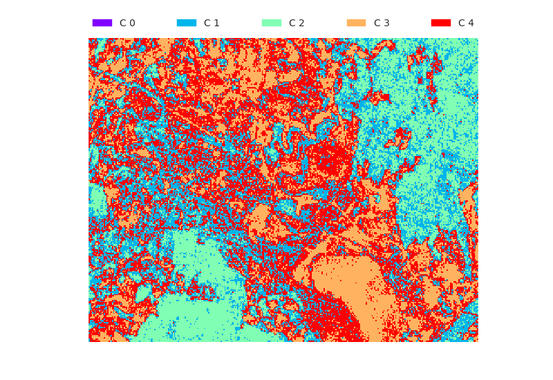
Evaluation results

Agreement with provided tm_classres.mat: $48.23 \%$ equally classified pixels.

Confusion matrix:

$\begin{array}{cc|rrrr} & & \rlap{\text{Proposal}} \\ & \text{Class} & 1 & 2 & 3 & 4 \\ \hline & 1 & 416 & 7 & 412 & 894 \\ & 2 & 976 & 1816 & 0 & 32 \\ \text{Reference} & 3 & 3 & 0 & 1647 & 329 \\ & 4 & 196 & 4 & 287 & 1118 \\ \end{array}$

Measure	Class 1	Class 2	Class 3	Class 4
RP	1,729	2,824	1,979	1,605
RN	6,408	5,313	6,158	6,532
PP	1,591	1,827	2,346	2,373
PN	6,546	6,310	5,791	5,764

TP	416	1,816	1,647	1,118
FP	1,175	11	699	1,255
FN	1,313	1,008	332	487
TN	5,233	5,302	5,459	5,277

tpr	0.24	0.64	0.83	0.70
tnr	0.82	1.00	0.89	0.81
ppv	0.26	0.99	0.70	0.47
npv	0.80	0.84	0.94	0.92
acc	0.69	0.87	0.87	0.79
iou	0.14	0.64	0.62	0.39
dsc	0.25	0.78	0.76	0.56
auc	0.53	0.82	0.86	0.75

Two feature images

Here we are using feature images tm1.png, and tm2.png.

Figure 1.7 Posterior images.

Figure 1.8 Classification result.

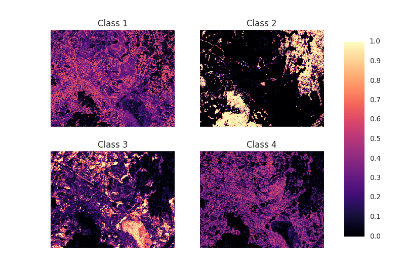
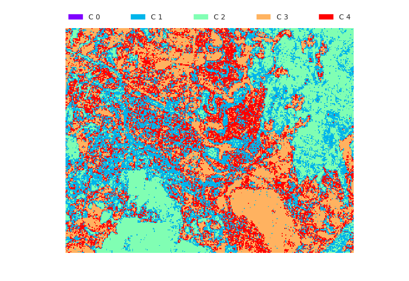
Evaluation results

Agreement with provided tm_classres.mat: $53.74 \%$ equally classified pixels.

Confusion matrix:

$\begin{array}{cc|rrrr} & & \rlap{\text{Proposal}} \\ & \text{Class} & 1 & 2 & 3 & 4 \\ \hline & 1 & 675 & 3 & 387 & 664 \\ & 2 & 735 & 2081 & 2 & 6 \\ \text{Reference} & 3 & 37 & 0 & 1830 & 112 \\ & 4 & 439 & 2 & 191 & 973 \\ \end{array}$

Measure	Class 1	Class 2	Class 3	Class 4
RP	1,729	2,824	1,979	1,605
RN	6,408	5,313	6,158	6,532
PP	1,886	2,086	2,410	1,755
PN	6,251	6,051	5,727	6,382

TP	675	2,081	1,830	973
FP	1,211	5	580	782
FN	1,054	743	149	632
TN	5,197	5,308	5,578	5,750

tpr	0.39	0.74	0.92	0.61
tnr	0.81	1.00	0.91	0.88
ppv	0.36	1.00	0.76	0.55
npv	0.83	0.88	0.97	0.90
acc	0.72	0.91	0.91	0.83
iou	0.23	0.74	0.72	0.41
dsc	0.37	0.85	0.83	0.58
auc	0.60	0.87	0.92	0.74

Four feature images

Here we are using feature images tm1.png, tm2.png, tm3.png, and tm4.png.

Figure 1.9 Posterior images.

Figure 1.10 Classification result.

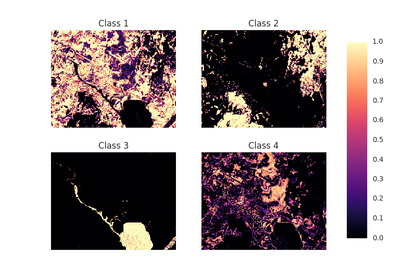
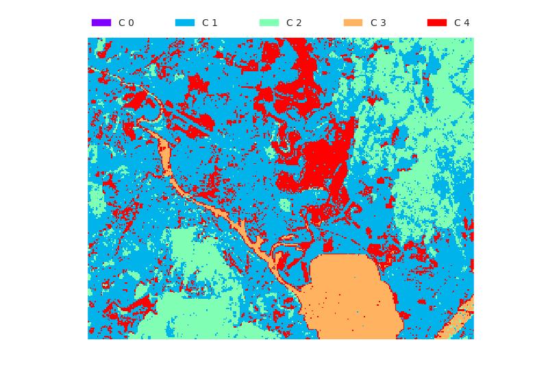
Evaluation results

Agreement with provided tm_classres.mat: $91.64 \%$ equally classified pixels.

Confusion matrix:

$\begin{array}{cc|rrrr} & & \rlap{\text{Proposal}} \\ & \text{Class} & 1 & 2 & 3 & 4 \\ \hline & 1 & 1466 & 4 & 5 & 254 \\ & 2 & 659 & 2163 & 0 & 2 \\ \text{Reference} & 3 & 3 & 0 & 1946 & 30 \\ & 4 & 198 & 2 & 0 & 1405 \\ \end{array}$

Measure	Class 1	Class 2	Class 3	Class 4
RP	1,729	2,824	1,979	1,605
RN	6,408	5,313	6,158	6,532
PP	2,326	2,169	1,951	1,691
PN	5,811	5,968	6,186	6,446

TP	1,466	2,163	1,946	1,405
FP	860	6	5	286
FN	263	661	33	200
TN	5,548	5,307	6,153	6,246

tpr	0.85	0.77	0.98	0.88
tnr	0.87	1.00	1.00	0.96
ppv	0.63	1.00	1.00	0.83
npv	0.95	0.89	0.99	0.97
acc	0.86	0.92	1.00	0.94
iou	0.57	0.76	0.98	0.74
dsc	0.72	0.87	0.99	0.85
auc	0.86	0.88	0.99	0.92

All feature images

Here we are using all feature images tm1.png, tm2.png, tm3.png, tm4.png, tm5.png, and tm6.png.

Figure 1.11 Posterior images.

Figure 1.12 Classification result.

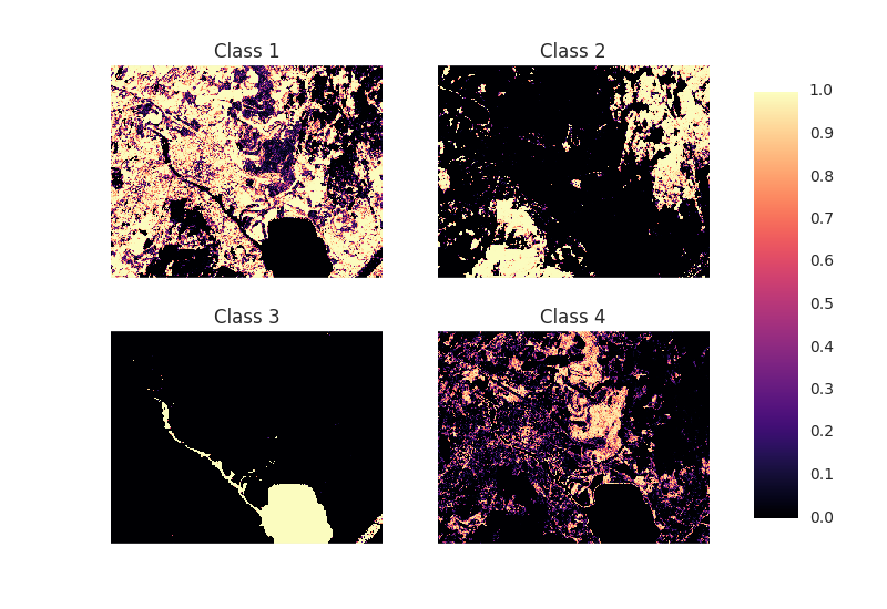
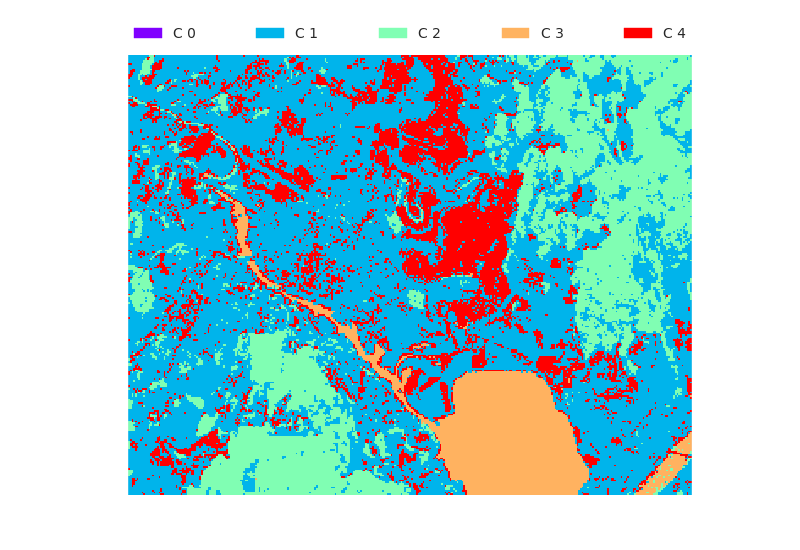
Evaluation results

Agreement with provided tm_classres.mat: $100.00 \%$ equally classified pixels.

Confusion matrix:

$\begin{array}{cc|rrrr} & & \rlap{\text{Proposal}} \\ & \text{Class} & 1 & 2 & 3 & 4 \\ \hline & 1 & 1474 & 3 & 1 & 251 \\ & 2 & 513 & 2311 & 0 & 0 \\ \text{Reference} & 3 & 14 & 0 & 1953 & 12 \\ & 4 & 213 & 2 & 0 & 1390 \\ \end{array}$

Measure	Class 1	Class 2	Class 3	Class 4
RP	1,729	2,824	1,979	1,605
RN	6,408	5,313	6,158	6,532
PP	2,214	2,316	1,954	1,653
PN	5,923	5,821	6,183	6,484

TP	1,474	2,311	1,953	1,390
FP	740	5	1	263
FN	255	513	26	215
TN	5,668	5,308	6,157	6,269

tpr	0.85	0.82	0.99	0.87
tnr	0.88	1.00	1.00	0.96
ppv	0.67	1.00	1.00	0.84
npv	0.96	0.91	1.00	0.97
acc	0.88	0.94	1.00	0.94
iou	0.60	0.82	0.99	0.74
dsc	0.75	0.90	0.99	0.85
auc	0.87	0.91	0.99	0.91

Equal variance

Here we are using all feature images tm1.png, tm2.png, tm3.png, tm4.png, tm5.png, and tm6.png. But contrary to the examples above, we assume independent features with equal variances, and equal class variance. With this, the covariance matrix becomes

$\Sigma_c = \Sigma = \sigma^2 I.$

In order to estimate the variance, I chose the unbiased least square, pooled variance estimator (see e.g. wikipedia)

$\hat{\sigma^2} = \frac{\sum_c\sum_x (n_{cx} - 1)\hat{\sigma_{cx}^2}}{\sum_c\sum_x (n_{cx} - 1)},$

where $n_{cx}$ is the number of training examples for feature $x$ in class $c$ , and

$\hat{\sigma_{cx}^2} = \frac{1}{n_{cx} - 1} \sum_i (x_{ci} - \hat{\mu_{ci}})^2$

is the variance for each feature $x$ in each class $c$ , and $x_{ci}$ is the feature value (not vector) in class $c$ . Note that, since in this example the priors are assumed uniform over the classes, we do not actually need to compute the variance estimate.

Figure 1.11 Posterior images.

Figure 1.12 Classification result.

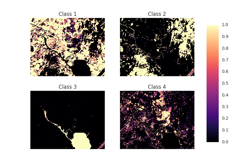
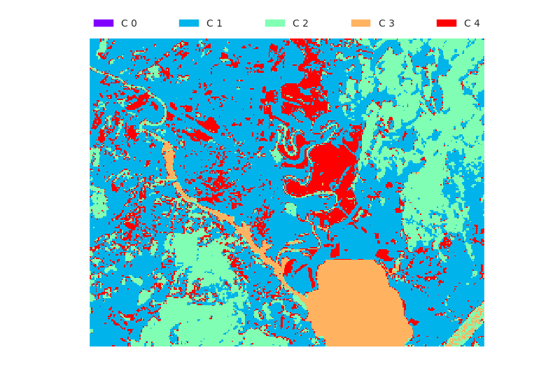
Evaluation results

Agreement with provided tm_classres.mat: $84.25 \%$ equally classified pixels.

Confusion matrix:

$\begin{array}{cc|rrrr} & & \rlap{\text{Proposal}} \\ & \text{Class} & 1 & 2 & 3 & 4 \\ \hline & 1 & 1373 & 16 & 6 & 334 \\ & 2 & 519 & 2275 & 1 & 29 \\ \text{Reference} & 3 & 1 & 0 & 1968 & 10 \\ & 4 & 314 & 15 & 0 & 1276 \\ \end{array}$

Measure	Class 1	Class 2	Class 3	Class 4
RP	1,729	2,824	1,979	1,605
RN	6,408	5,313	6,158	6,532
PP	2,207	2,306	1,975	1,649
PN	5,930	5,831	6,162	6,488

TP	1,373	2,275	1,968	1,276
FP	834	31	7	373
FN	356	549	11	329
TN	5,574	5,282	6,151	6,159

tpr	0.79	0.81	0.99	0.80
tnr	0.87	0.99	1.00	0.94
ppv	0.62	0.99	1.00	0.77
npv	0.94	0.91	1.00	0.95
acc	0.85	0.93	1.00	0.91
iou	0.54	0.80	0.99	0.65
dsc	0.70	0.89	1.00	0.78
auc	0.83	0.90	1.00	0.87

Task 2

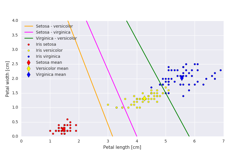
Given the mean value for each class, the decision boundary between two classes using a minimum distance classifier is the line containing all points that are equidistant to the two class means.

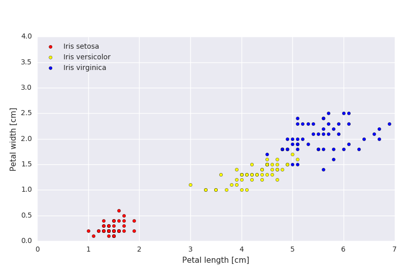
By using the actual data from the Iris flower data set from Ronald Fisher (see more here), we can compute the actual means and decision boundaries.

Figure 2.1 Fisher's Iris flower data set.

Figure 2.2 Fisher's Iris flower data set with drawn means and decision boundaries.

Task 3

A classifier that uses Euclidean distance, computes the distance from point $x$ to class $c$ as

$D_c(x) = || x - \mu_c ||_2.$

Classification with this rule is equivalent to using the discrimination function

$d(x) = \arg\max_c \left\{ x^\intercal \mu_c - \frac{1}{2}\mu_c^\intercal \mu_c \right\}$

That is we associate point $x$ with the class $c$ that has a class mean closest to the point, therefore we get a discrimination function

$\begin{align} d(x) &= \arg\min_c \left\{ || x - \mu_c ||_2 \right\} \\[0.5ex] &= \arg\min_c \left\{ || x - \mu_c ||_2^2 \right\} \\[0.5ex] &= \arg\min_c \left\{ (x - \mu_c )^\intercal (x - \mu_c) \right\} \\[0.5ex] &= \arg\min_c \left\{ x^\intercal x - x^\intercal \mu_c - \mu_c^\intercal x + \mu_c^\intercal \mu_c \right\} \\[0.5ex] &= \arg\min_c \left\{ - 2x^\intercal \mu_c + \frac{1}{2}\mu_c^\intercal \mu_c \right\} \\[0.5ex] &= \arg\min_c \left\{ - x^\intercal \mu_c + \frac{1}{2}\mu_c^\intercal \mu_c \right\} \\[0.5ex] &= \arg\max_c \left\{ x^\intercal \mu_c - \frac{1}{2}\mu_c^\intercal \mu_c \right\}, \end{align}$

which is what we were asked to show.

Task 4

Assuming equal class prior $p$ and gaussian likelihood with class mean $\mu_c$ and equal covariance matrix $\Sigma$ for each class $c$ , the discrimination function becomes (see the notes

$\begin{align} d(x) &= \arg\max_c \left\{f_{C|X = x}(c) \right\} \\[0.5ex] &= \arg\max_c \left\{ x^\intercal \mu_c - \frac{1}{2}\mu_c^\intercal \Sigma^{-1} \mu_c \right\}. \end{align}$

Now, for a $2\times 2$ , invertible matrix

$A = \left( \begin{array}{cc} a_{11} & a_{12} \\ a_{21} & a_{22} \end{array} \right)$

the inverse matrix is given by

$A^{-1} = \frac{1}{\det (A)} \left( \begin{array}{cc} a_{22} & -a_{12} \\ -a_{21} & a_{11} \end{array} \right)$

where the determinant is computed as

$\det(A) = a_{11}a_{22} - a_{12}a_{21}.$

This can be checked via the definition $A A^{-1} = I$ , where $I$ is the identity matrix.

a)

In our case,

$\Sigma = \left( \begin{array}{cc} 1.2 & 0.4 \\ 0.4 & 1.8 \end{array} \right)$

making the inverse equal to

$\Sigma^{-1} = \frac{1}{2} \left( \begin{array}{cc} 1.8 & -0.4 \\ -0.4 & 1.2 \end{array} \right).$

The class means are

$\mu_1 = \left( \begin{array}{c} 0.1 \\ 0.1 \end{array} \right), \quad \mu_2 = \left( \begin{array}{c} 2.1 \\ 1.9 \end{array} \right) \quad \mu_3 = \left( \begin{array}{c} -1.5 \\ 2.0 \end{array} \right),$

which, when we compute the discrimination function for each class mean, the feature vector

$x = \left( \begin{array}{c} 1.6 \\ 1.5 \end{array} \right)$

is classified to class 2.

b)

Given a collection of points with mean vector $\mu$ and covariance matrix $\Sigma$ , the Mahalanobis distance from a point $x$ to the set of points is given by

$d_M(x) = \sqrt{(x - \mu)^\intercal \Sigma^{-1} (x - \mu)}.$

Using the covariance matrix above, and with a mean vector

$\mu = \left( \begin{array}{c} 2.1 \\ 1.9 \end{array} \right)$

the distance plot (with contour lines) is

Figure 4.1 Mahalanobis distance.

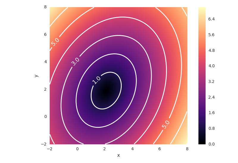
This could also have been found by computing the eigenvectors $v_i$ and eigenvalues $\lambda_i$ (for $i \in \{1, 2\}$ ) of the covariance matrix

$(\Sigma - \lambda_i I)v_i = 0.$

All points on the ellipse with major and minor axis proportional to the largest and smallest eigenvalue of $\Sigma$ , and which orientation is given by the corresponding eigenvectors, will then have an equal Mahalanobis distance from the mean vector (and thus constitute the contours shown in Figure 4.1, for different distances).

Task 5

This task is similar to Task 4 a), just with different class means and feature vector. The feature vector is classified as class 1.